Demo: Displays of Technical Indicators
(Revised September 10, 2006)
This demonstration explains the different QuanTek technical indicators, and explains the calculation of the Momentum indicators and Trading Rules. There are three different basic types of indicator, which are called Relative Price, Velocity, and Acceleration. These three types correspond to the number of derivatives (rates of change) taken by the (acausal) Savitzky-Golay smoothing filter. The Relative Price indicator corresponds to no derivatives, and is just the difference between smoothed (log) prices with two different time scales of smoothing, with various time lag settings. In fact, for each of the three types you can take a difference between two smoothings with different time scales and time lags, but for the Relative Price indicator this is essential, since the (log) prices themselves do not fluctuate around zero. For this indicator alone, if you do not choose a second indicator, the 512-day smoothing is chosen by default. If you choose a time scale for smoothing of zero, the raw (log) prices are used. The Velocity indicator is the first derivative, or rate of change, of the price. This is calculated digitally by the smoothing filter, but corresponds to the returns. In fact, if you choose a time scale of zero, the Velocity is precisely the one-day returns. The Acceleration is the second rate of change of the price. For time scale zero, it is the second difference of the price. So you can choose any of these three types, with any smoothing time scale from 1 to 512 days, and any time lag from -100 to +100 days. And you can choose a difference between two such smoothings. This gives a very wide range of possible technical indicators, covering just about all possibilities for linear oscillator-type indicators involving price alone. Note that these three types are precisely the ones in the Harmonic Oscillator indicator, which is a simple acausal smoothing of the price data with no time lag and a smoothing time scale the same as the time horizon (set in the Trading and Portfolio Parameters dialog). The Harmonic Oscillator indicators are quick to compute and provide visual reference points in the form of the buy/sell points, but the Momentum indicators can actually be tested for correlation with future returns using the QuanTek statistical tests.
When the Momentum indicators are not current, they are not displayed, otherwise the N-day forward averaged Momentum indicators are displayed in the Momentum indicators splitter window. The weighted sum of these indicators is called the N-day forward averaged Trading Rules indicator, and is displayed in the Trading Rules splitter window, bottom pane. The actual forward averaged returns, averaged over the time horizon, are displayed just above the Trading Rules indicator for comparison. This is because the Trading Rules indicator for time horizon of N days is supposed to be correlated with the N-day future returns, or returns forward averaged over N days. To design and compute the Momentum indicators, for each stock, you open the stock data file and use the Technical Indicators dialog and the Correlation Test - Indicators dialogs together. You can switch back and forth between these using a button in each dialog. Before you start, however, you must calculate a set of 1024 Price Projections, one for each day in the past going back 1024 days. You can do this by clicking the Calculate (Stock) Data button on the toolbar, when a security data file is open. This also calculates the Momentum indicators and Trading Rules indicator using the current saved settings, so that they are displayed in their splitter windows. If you just want to use the existing settings, this is all you have to do to update these indicators. If the Momentum and Trading Rules indicators are current, then they are displayed in their splitter windows, and if they are not current then these windows are blank.
Price Projection
The Main Graph for AAPL stock is shown here. There are actually 4 different scales, labeled 1, 2, 4, 8; the scale shown here is scale 2. The past prices are shown in white (with the black background), and the Price Projection from the Linear Prediction filter is shown in blue. Also shown are one standard deviation error bars for the Price Projection, calculated as if it were a Random Walk. The green/red arrows are the recommended buy/sell points corresponding to the chosen time horizon (10 days here). The yellow curve is a 512-day Savitzky-Golay smoothing, and the sets of curves on either side of it are one-standard deviation and two-standard deviation (with this time horizon) Bollinger Bands. The relative log volume is shown along the bottom, relative to the average log volume.
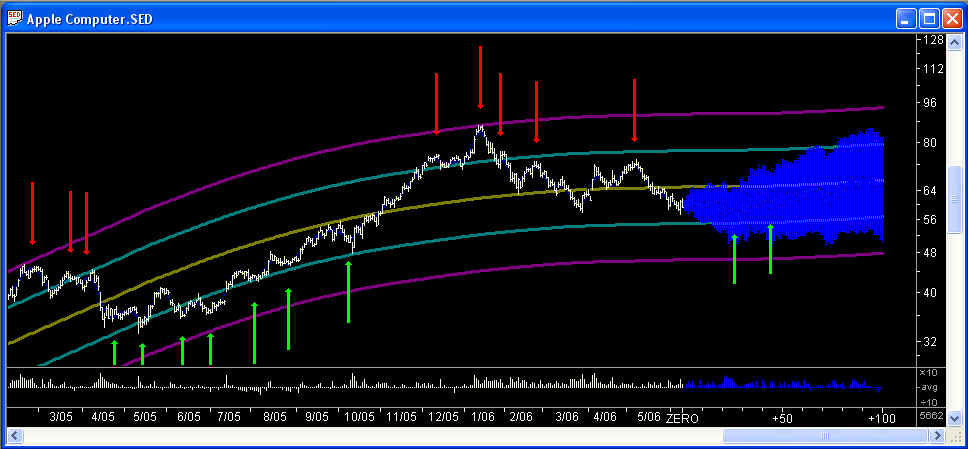
The Price Projection itself is perhaps the most important technical indicator, of course. The validity of this Price Projection can be tested using the Correlation Test - Filters dialog, which is available within the Hybrid LP Filter dialog (on the Greeting dialog or Main toolbar). You can also set the filter type and filter parameters for the Linear Prediction filter for each security data file separately in the Hybrid LP Filter dialog. (Note: The filters that seem to work best are the Discrete Wavelet Transform (DWT) filters, and the Price Projection from these have a smoother appearance than that shown above, which is a Fast Fourier Transform (FFT) filter.)
The main purpose of the Price Projection is to try to estimate the future returns of the price over the longer term, from say 10 days up to 100 days. It is these longer-term price moves, corresponding to the low-frequency end of the spectrum of the returns, which we expect to have the greatest degree of "predictability". These are also the price moves that are most important for calculating the optimal portfolio. The shorter term moves, up to 10 days or so with daily data, appear to be mostly stochastic noise which has the effect of masking whatever correlation exists in the data. Most of the spectral power lies in these high-frequency modes as well; in fact the modes from 2 to 4 days contain half the spectral power (where 2 days is the Nyquist frequency, which is the highest possible frequency). So the strategy is to try to filter the high-frequency modes out using the Savitzky-Golay digital smoothing filter, then use the remaining low-frequency modes as the basis of a set of technical indicators. In this way we hope to establish a positive correlation between these technical indicators and future returns, thereby demonstrating their effectiveness.
Harmonic Oscillator Indicators
For each security data file, a set of Harmonic Oscillator indicators is computed each time the data file is opened. These are simple acausal smoothings using the Savitzky-Golay smoothing filter, of the past price data together with the future Price Projection. The entire graph depends only on data up to the present day, which is marked by a vertical yellow line at the ZERO point, so relative to the present day, the Harmonic Oscillator indicator is causal. However, relative to each past day the acausal smoothing uses data points both to the past and future of that day, so for each of the past days the Harmonic Oscillator indicator is acausal. The indicated buy/sell points for the past days are therefore with the "benefit of hindsight". The purpose of this is to illustrate the nature of the buy/sell points on the graphs for a given setting of the time horizon, and also to provide a convenient set of reference points to line up features on all the graphs, including the Main Graph. The buy/sell points for the future days are estimated based on the Price Projection, which itself uses only data up to the present, so these buy/sell points are causal. As these buy/sell points approach the ZERO line, they may be used as buy/sell recommendations for the given time horizon for trading.
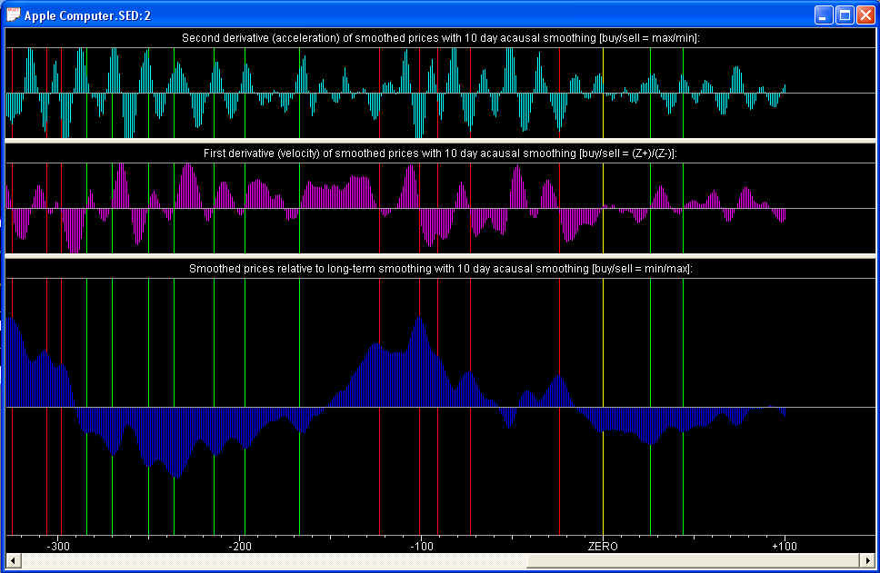
In the Harmonic Oscillator splitter window, you can see the three technical indicators that make up the Harmonic Oscillator indicator. The bottom indicator, called the Relative Price, is the N-day smoothed price relative to the 512-day smoothed Reference Curve (yellow curve on the Main Graph), where the smoothing time scale N is the time horizon. Above it is the Velocity indicator, which is the rate of change of the Relative Price. It shows the slope, or rate of change, of the N-day smoothed price (relative to the Reference Curve). The top indicator is the Acceleration, which shows the rate of change of the Velocity, and the curvature of the Relative Price. This indicator shows the turning points of the Relative Price; positive curvature for a buy point and negative curvature for a sell point.
Through all three graphs you will note green and red vertical lines. These correspond to the buy/sell points displayed on the Main Graph. The buy/sell points correspond to the first of a series of buy/sell signals. These in turn are defined in terms of the Harmonic Oscillator indicators as follows: A buy signal occurs whenever the Relative Price is negative (and below a certain Range level set in the Trading and Portfolio Parameters dialog), the Velocity is positive, and the Acceleration is positive. A sell signal occurs whenever the Relative Price is positive (and above a certain Range level set in the Trading and Portfolio Parameters dialog), the Velocity is negative, and the Acceleration is negative. Thus you will note that the green buy points pass through the minima (min) of the Relative Price indicator, the upward crossing zero points (Z+) of the Velocity indicator, and the maxima (max) of the Acceleration indicator. The red sell points pass through the maxima (max) of the Relative Price indicator, the downward crossing zero points (Z-) of the Velocity indicator, and the minima (min) of the Acceleration indicator. The crossing points are specified in the label for each graph, as a reminder. These buy/sell points serve to line up the features on all the different QuanTek graphs. The buy/sell signals are shown on the two highest scales of the Main Graph. These signals are located in price at a point which is below/above the N-day smoothing of the price; the degree to which these signals are below/above the smoothed price is controlled by the Threshold level set in the Trading and Portfolio Parameters dialog. The purpose of the buy/sell signals is to serve as recommended points to set buy/sell limit orders. These buy/sell signals for the present day are also listed for each security in the Short-Term Trades dialog.
Momentum Indicators
Here is shown the Momentum Indicators splitter window. In the three panes of this splitter window are displayed the three Momentum indicators that you design yourself using the Technical Indicators dialog box, and test for correlation with future returns using the Correlation Test - Indicators dialog. Generally, the Momentum 0 indicator will be a Relative Price, the Momentum 1 indicator will be a Velocity, and the Momentum 2 indicator will be an Acceleration. However, you can choose any of the three types you wish for each of the three indicators.
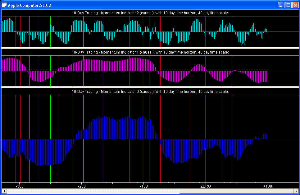
You will notice that there is a very rough correspondence or correlation between the three indicators. This correlation is certainly not perfect by any means. But bear in mind that it takes only a very small degree of correlation between the technical indicators and future returns to be able to make very rewarding returns from short-term trading. In the indicators above, the time scale is 40 days while the time horizon is only 10 days, and the large-scale fluctuations of the stock data are more like 100 days in duration. So with these settings there is no close correspondence apparent between the large-scale fluctuations and the buy/sell points. Nevertheless, if you were to adjust your position at the buy/sell points in proportion to the above 10-day forward averaged Momentum indicators, then theoretically you should make a good return on your trades because these indicators are positively correlated with the 10-day future returns, as shown by the Correlation Test - Indicators dialog.
Actually, if you compare the Momentum indicators with the Harmonic Oscillator Relative Price indicator, you will see that the Momentum indicator is positive roughly during the 100-day interval in which the Relative Price indicator is in a slow overall uptrend. This is precisely the period in which you want to be long in your position, while the slope of the Relative Price is positive. The buy/sell points, on the other hand, occur when the Relative Price is negative/positive respectively. (You buy or sell before the price enters an uptrend or downtrend!) Notice that the buy/sell points actually correspond, roughly, to that portion of the Momentum indicator that is making a transition from negative to positive or positive to negative, respectively, or the portion before making the transition. These are the periods when the position should be going from short to long or long to short, respectively. So the phase of the Momentum with respect to the Relative Price is actually correct, if the trading position is supposed to be proportional to the value of the Momentum indicator (assuming the position to be held for 10 days, more or less). Once again, the agreement is not perfect, but any correlation at all can lead to very profitable short-term trading! Remember, the Random Walk model says that it is impossible to find any technical indicator at all that has a positive correlation with future returns!
Trading Rules Indicators
A third splitter window is called the Trading Rules splitter window, because the Trading Rules indicator is in the bottom pane. This is the N-day forward averaged Trading Rules indicator, which is supposed to be correlated with the N-day future returns, which are actually N-day forward averaged . Therefore, this latter N-day forward averaged returns, both future (projected) and past, is shown in the pane just above the Trading Rules. Theoretically, and by design, the two should be correlated and hence in phase, at least approximately. At the top is a Volatility indicator, also N-day forward averaged.
The Trading Rules indicator is a sum of the three Momentum indicators, with weights that you choose in the Trading Rules Parameters dialog. The Returns are the difference in the close-to-close log prices, forward averaged. The Volatility is the absolute value of the high minus low difference in daily log prices, also forward averaged. So all three indicators in this splitter window are N-day forward averaged, for easy comparison.
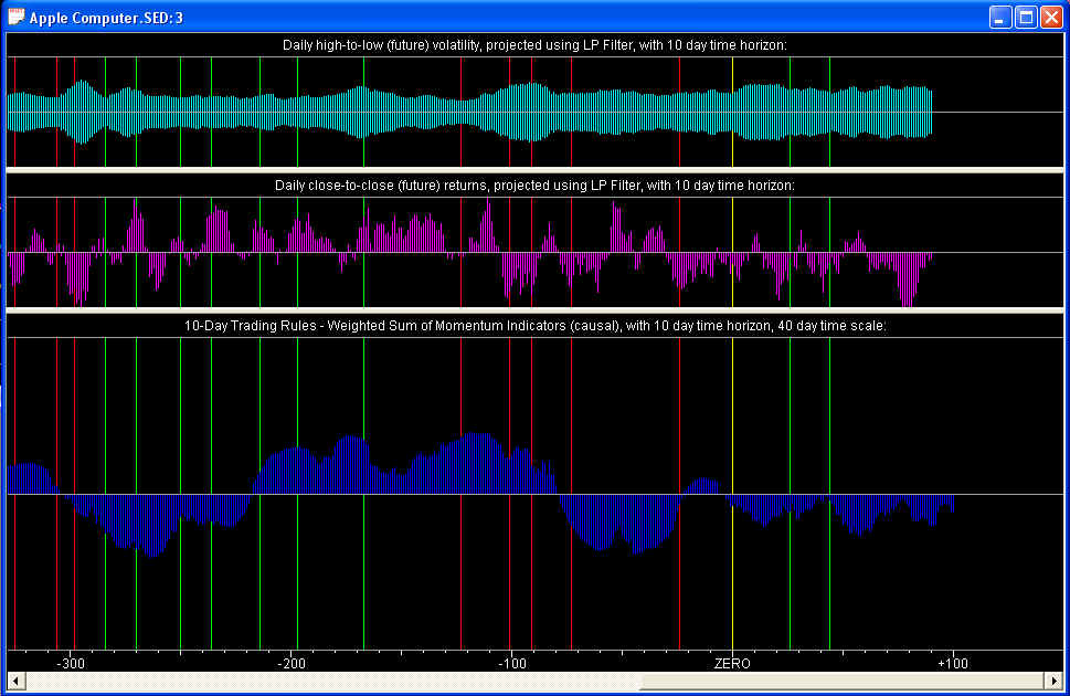
In the above graph, it is hard to see any correlation between the Trading Rules in the lower pane, and the Returns in the second pane. Part of this could be due to the use of the 40-day time scale for the Momentum indicators, which seems to have nothing to do with any natural time scale of the price swings of this particular stock. But the correlation could exist, and lead to profitable short-term trading, without it being readily apparent and visible to the eye. It is the purpose of the Correlation Test - Indicators to measure this correlation precisely, just because it may not be at all apparent by visual inspection.
The N-day Trading Rules are designed to have a positive correlation with the N-day future returns. So the relative value of the Trading Rules indicator should be an indicator of the expected returns over the next N days. Thus to use this indicator, you can adjust your position according to the Trading Rules indicator, then hold this position for the next N days, where N is the time horizon for trading. You can then use the N-day buy/sell points as the recommended times to adjust your position, and adjust the amount of the position in accordance with the Trading Rules indicator. The value of the Trading Rules indicator for the present time is shown in the Short-Term Trades dialog. You can also view a graph of the Trading Rules indicator, along with the Momentum indicators, with a calibrated vertical scale, by calling up the Technical Indicators dialog.
Normalization of Trading Rules
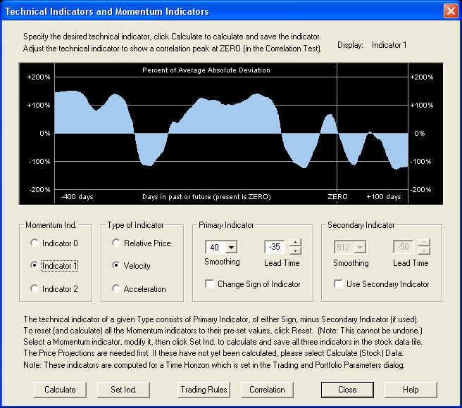
The Momentum indicators and Trading Rules indicators can be viewed in their respective splitter windows, but they can also be viewed within the Technical Indicators dialog itself. The display in the Technical Indicators dialog has a scale ranging from -200% to +200%, unlike the splitter windows which have no scale. So to find the actual numerical value of the indicators, you can look at them in the Technical Indicators dialog. The scale has the interpretation that the percentage indicates the relative percentage invested of the trading equity allocated for short-term trading in this individual stock. It can be interpreted as analogous to the margin leverage for trading in this individual stock, with the given equity. So if the Trading Rules indicator is at +100%, this means a recommendation of being fully invested on the long side, while +200% means fully extended on margin, and likewise for negative percentages on the short side. This being the case, it should be explained how the Momentum indicators and Trading Rules indicator are normalized. First the average absolute value of each Momentum indicator is measured, and this value corresponds to the average absolute percentage of the equity invested of 100%. Then, given this value, the Momentum indicators are passed through a certain non-linear function, which "compresses" their peak values, and these peak values are then limited to an absolute value of approximately 158%. So this is the maximum "margin leverage" for each individual Momentum indicator. But the three Momentum indicators are added together, with weights you can adjust from 0% to 100%, to form the Trading Rules indicator. Since the three Momentum indicators should be roughly in phase (if they have been properly designed), at their peaks the peak values would be 474% if all three settings of the weights are on their maximum values of 100%. So this sum was divided by two so that the absolute maximum "margin leverage" with the weights all set to 100% will be 237%. More likely the peaks will be close to approximately 200% with the three weights all set to 100%. If the weights are set to their middle value of 50%, then the peaks of the Trading Rules indicator will reach a maximum absolute value of approximately 100%, which means all of the allocated equity is invested, but you are not yet extended on margin. So to measure the actual percentage value of the Trading Rules or Momentum indicators, please look at them in the Technical Indicators dialog. Note that the current value of the Trading Rules indicator is also shown in the Short-Term Trades dialog. This will be the value under the ZERO line in the Technical Indicators dialog graph when the Trading Rules are displayed.
Shown here is the Technical Indicators dialog, with the Momentum 1 indicator displayed, which is a Velocity indicator. (Compare this to the Momentum 1 indicator displayed above in the splitter window. They are the same, except for the expanded horizontal scale in the splitter window.) Notice that its peaks are somewhat "flattened", and the peak values are +158% and -158% (except possibly for the future projected part, which is merely "cosmetic" anyway). The important value is the one under the ZERO line, which is the current recommended N-day position for short-term trading:
To view any of the three Momentum indicators (assuming they have already been saved), you can click on any one of the three radio buttons in the Momentum Ind. group. The selected Momentum indicator will be displayed in the graph. To view the Trading Rules indicator, click on the Trading Rules button. This brings up the Trading Rules Parameters dialog, from which you can set the three weights which define the Trading Rules as a sum of the three Momentum indicators (for each security). When you close this dialog, these settings are saved. Then the Trading Rules indicator is displayed in the graph. This graph has an advantage over the splitter windows in that it is calibrated on the vertical scale. So you can see at a glance the actual value of the Momentum and Trading Rules indicators, in terms of the recommended margin leverage to use for a short-term trading position in the given security. Again, the value of the Trading Rules indicator under the ZERO line (present time) is also displayed in the Short-Term Trades dialog.
Calculation of Technical Indicators
To calculate the Momentum indicators, you must first calculate a set of 1024 Price Projections, using Calculate (Stock) Data in the Main Graph toolbar for each security data file. The Calculate (Stock) Data routine works in the following way. The objective is to compute a set of technical indicators which are causal in the sense that for each day, the indicators for that day use only data of that day or to the past of that day -- no future data are allowed! So for each day in the past, going back 1024 days, the Price Projection is calculated with that day taken as the present day. Thus the Price Projection relative to that day itself is a (linear) function only of the price returns for that day or earlier -- no later data enter the Price Projection. Then each of these 1024 data sets consisting of the price data to the past (or present, not future) of day N together with its Price Projection relative to that day, are smoothed using the Savitzky-Golay smoothing filter. You can select any of the choices outlined above for this smoothing, noting especially the time scale setting, which is just the smoothing time scale for the filter (not to be confused with the time horizon for trading). Now we have a set of 1024 smoothing curves, each one using only data to the past or present of day N, where N ranges from 0 to 1024 days in the past. Now, each of these smoothing curves is indexed the same way as the curves on the main graph, going from, say, 1024 days in the past (relative to day N) to 100 days in the future. Call this index K -- it is identified with the time lag or lead time. (Hence we actually need 2048 days of price data to calculate a complete set of data for the Momentum indicators.) Then for each value of K, we actually have a separate technical indicator that we can use for trading rules. Changing the setting of the lead time sets a value of K, and for each N the value of the smoothing curve for index K is taken as the value of the technical indicator with index N. Then by construction, the value of the technical indicator with index N depends only on past or present data, relative to day N -- no future data! So what we have constructed is a causal technical indicator, in fact, a whole set of such indicators labeled by the lead time K. Given the value of K, then, this technical indicator is graphed (in the Momentum indicators splitter window), with the index of each value of the indicator corresponding to the index N, and each such value of the indicator depends on price data to the past or present of day N. (The indicator is then projected into the future using a generic Linear Prediction filter, but it is the value of the indicator for day 0 -- the present day -- that is of greatest interest.)
We may now calculate correlations by taking a certain point, labeled by index K, on each smoothing curve N, and computing the correlation between this point (taken as the value of our technical indicator) and the future returns relative to day N. Each point on curve N uses only data to the past or present of day N, and the correlation is taken with future returns to the future of day N, so this ensures that there can be no mixing up of future data with past data. This correlation is computed, as a function of the lead time K, and displayed as a graph in the Correlation Test - Indicators dialog, with K along the horizontal axis and the correlation along the vertical axis. In this dialog you can measure which lead time corresponds to maximum correlation, by moving the graph back and forth using the Lead Time spin indicator until the correlation peak is under the ZERO line. Then this value of Lead Time corresponding to maximum correlation is used to adjust (automatically) the Lead Time setting in the Technical Indicators dialog, which is the setting of the index K described above. Note that the Lead Time setting in the Technical Indicators dialog selects the index K, and hence selects a different technical indicator for each setting of the Lead Time. The correlation of the indicator with future returns for each setting of the lead time (from -100 days to +100 days) is displayed on the graph in the Correlation Test - Indicators dialog, and the Lead Time setting in this dialog merely moves the graph back and forth to move the correlation peak under the ZERO line and hence choose the optimum value for the lead time. So this is the connection between the two Lead Time controls. This Lead Time setting is crucial, because it is necessary to adjust the phase of the technical indicator for maximum correlation with future returns.
Traditional Technical Indicators
The Harmonic Oscillator indicator is now considered again, and each component compared to the traditional technical indicator to which it is most similar.
N-day Smoothing:
Moving Averages: The N-day smoothing of the price graph is, of course, similar to a (simple) moving average. The main difference is that the smoothing uses both past and future data, and has no time delay, unlike the moving average, which uses only past data. Close to the present day, the smoothed data must make use of the future projected prices from the Price Projection routine. Also, the Savitzky-Golay digital smoothing filter preserves the shape of features with a period longer than N days, better than the moving average. The difference of two smoothings with different time periods may be used in a similar fashion to the difference of two moving averages, except for the fact that there is no time delay in the smoothing. So if the price is trending uniformly upward or downward, the two smoothed price curves will not lead or lag one another (unlike the two moving averages). In the case of two moving averages, this time delay means that the difference of the two moving averages functions similarly to a derivative of the price curve (Velocity). The difference of two smoothings may be used to indicate a short-term fluctuation relative to a longer-term average, but since there is no time delay the difference does not function as a derivative. On the other hand, derivatives may be calculated from the Savitzky-Golay digital smoothing filter directly.
Relative Price:
Moving Average Convergence Divergence (MACD): The standard MACD indicator is the difference of two exponentially weighted moving averages, the slower moving average of 130 trading days, and the faster one of 60 days. The difference is then smoothed by a 45 day moving average. This is somewhat similar to what is done in the Relative Price indicator, except that the Savitzky-Golay digital smoothing filter is used instead of exponentially weighted moving averages, thereby eliminating the time lag. In the Relative Price indicator, with the trading time scale set to N days, the difference is taken between the N-day smoothed price and the Reference Curve consisting of the 512-day smoothed price. The result of this is that the short-term modes with periods less than N days are eliminated by the N-day smoothing, and the long-term modes with periods greater than 512 days are eliminated by subtracting the Reference Curve. This produces a type of oscillator, with no time lag, in which the predominant modes have periods close to N days. Of course, by constructing a Momentum indicator of the Relative Price type, a wide range of time scales and time lags may be used, not just the one particular choice specified in the traditional MACD indicator.
Williams' Percentage Range (Percentage R): This indicator takes the prices over the past N-day time interval, then plots the current price as a percentage of the price interval between the highest and lowest price within that time interval. It thus displays the current price within the trading range established over the past N days. This indicator is similar to one obtained by comparing the current price to the Relative Price indicator with N-day smoothing. Both indicators show when the price swings have reached oversold and overbought limits, indicating buy/sell points respectively. However, in QuanTek the emphasis is more on the longer-term price moves, so the price moves on a time scale equal to the time horizon N are normally compared to much longer-term price moves. However, if you wish you can design a Momentum indicator consisting of a difference of two smoothed prices, with the shorter-term smoothing of 0 (no smoothing) and the longer-term smoothing of N days, and this will be roughly similar to the Percentage R.
Velocity:
Oscillator: The traditional Oscillator of Technical Analysis is closely related to the Velocity part of the Harmonic Oscillator indicator of QuanTek . The traditional Oscillator is just the difference between the most recent closing price and the closing price N days ago, expressed as a point within the range of prices covered within the last N days. This range of prices is usually normalized to the interval between -1 and +1. But the traditional Oscillator can be seen to be the average price velocity over the past N days. The traditional Oscillator is intended to identify potential N-day minima and maxima in the price curve, corresponding to buy and sell points. It does this because the traditional Oscillator is a time delayed indicator, by an average of N/2 days, but the price velocity of a pure sine wave with a period of 2N leads the price curve of the sine wave by one quarter cycle, which is N/2 days. In this way the traditional Oscillator is supposed to be roughly in phase with the price curve itself. The N-day Oscillator will in general smooth out the price fluctuations with periods shorter than 2N days, for which a half cycle is N days, leaving the 2N day cycle as the shortest cycle. Then, since the velocity leads the prices by N/2 days but the traditional Oscillator lags the price data by that same amount, interpreting the Oscillator as representing the 2N-day cyclic price swings leads to an estimate of the buy/sell points. The Velocity part of the Harmonic Oscillator indicator measures the price velocity directly, with no time lag, so its buy/sell points are indicated by zero-crossing points corresponding to local minima and maxima of the price curve.
Wilder's Relative Strength Index (RSI): This index is also similar to the Velocity of the Harmonic Oscillator indicator in that both are related to the first derivative of the N-day smoothed prices. The Velocity indicator shows this directly, of course. The RSI indicator is a more indirect measure of the first derivative and is again lagged in time by N/2 days. The RSI indicator is constructed by counting the Ups and Downs over the N day interval. An Up is the difference in closing price on a certain day minus the closing price the day before, if this quantity is positive, and zero if it is negative. Likewise, a Down is the difference in closing prices if it is negative, expressed as the absolute value (a positive number), and zero if the difference is positive. The RSI is then defined as the sum of all the Ups divided by the total Ups plus Downs over the N-day interval, multiplied by 100. It thus ranges between zero and 100. (They should have defined it as (Ups - Downs)/(Ups + Downs), a number between -1 and +1, but oh well.) The RSI indicator actually contains essentially the same information as the traditional Oscillator described above, since the modified version of the RSI that was just suggested is virtually identical to the definition of the traditional Oscillator, provided we use the value of the Ups and Downs, not just the number. (The value of (Ups - Downs) is just the difference in closing prices between now and N days ago, and the value of (Ups + Downs) is roughly the expected range in prices over the N days.) However, the main difference seems to be that the RSI is a nonlinear function of past returns, in that it uses only the number of Ups and Downs, without regard to their actual value. Whether or not this nonlinearity is an advantage is questionable. This indicator was probably devised in the first place for the sake of ease of computation, before the era of the personal (or any other) computer.
Lane's Stochastics: This is a composite indicator consisting of the RSI indicator over a short time interval, together with three moving averages of this indicator. Actually, in Eng's book [Eng (1988)] the definition of this indicator is a little ambiguous, because although it is defined to use the RSI indicator, in the actual description of how to set up the indicator it sounds more like it uses a variation of the Percentage R indicator. However, there should not be a whole lot of difference between a short time period RSI indicator and the Percentage R indicator, so either will probably work. In both cases, the overbought signals are at the troughs of the indicator, and the oversold signals are at the peaks. To complete the Lane's Stochastics indicator, one takes a short time moving average of the RSI or Percentage R, then a moving average of that moving average, and finally another moving average of the second one. One plots the first two indicators together, and the last two indicators together, forming two separate graphs. The buy/sell points are indicated at the crossover points of the two moving averages in each graph. Note now that comparing two moving averages with different time scales is similar to the concept of taking a derivative, and the crossover points of the MAs correspond to the zero-crossing points of the derivative. If RSI is used, then this is effectively a way to determine a time-delayed second derivative of the prices, while if Percentage R is used; the result is effectively a first derivative of the prices that is not time-delayed. In either case, the crossover point is equivalent to the zero-crossing point of the Velocity of the Harmonic Oscillator indicator. So, instead of comparing two moving averages to effectively get the zero-crossing points of the first derivative of the price graph, it is much better to calculate this quantity directly by using the Savitzky-Golay smoothing filter to compute a Velocity indicator.
Acceleration:
Lane's Stochastics: None of the usual indicators seem to calculate a second derivative directly, although Lane's Stochastics calculates a kind of effective time-delayed second derivative if one mentally pictures the difference of two moving averages of the RSI indicator. However, it is much more straightforward to calculate this smoothed second derivative directly using the Savitzky-Golay smoothing filter to compute an Acceleration indicator.
Conclusion
To be honest, it appears that many of the standard technical indicators were devised before the days of personal computers, and were constructed the way they were because they were the only quantities that were easy to calculate by hand. The Price Projection, Harmonic Oscillator indicator, Momentum indicators, Trading Rules indicator, and other technical indicators in QuanTek evidently contain much more information and are easier to interpret than these standard technical indicators. The also have much more of a basis in the standard theory of Stochastic Time Series and Signal Processing. In addition, in the QuanTek program the Momentum indicators can be tested for correlation with future returns, thereby directly verifying their effectiveness as technical indicators.
References
Peter J. Brockwell & Richard A. Davis, Time Series:
Theory and Methods, 2nd ed., Springer-Verlag, New York (1991)
William F. Eng, The Technical Analysis of Stocks, Options, & Futures, McGraw-Hill, New York, NY (1988)
Edgar E. Peters, Chaos and Order in the Capital Markets,
John Wiley & Sons, Inc., New York, NY (1991)
Edgar E. Peters, Fractal Market Analysis, John Wiley & Sons, Inc., New York, NY (1994)
William H. Press, Saul A. Teukolsky, William T. Vetterling, & Brian P. Flannery (NR), Numerical Recipes in C, The Art of Scientific Computing, 2nd ed., Cambridge University Press, Cambridge, UK (1992)
return to Demonstrations page