Demo: Momentum Indicators - Design and Testing
(Revised November 13, 2006)
This demonstration outlines the steps for the design and testing of a custom Momentum indicator. You can design three Momentum indicators, which are supposed to be (linear) functions of the past data that show positive correlation with future returns, over an N-day time horizon. These linear functions are various types of smoothing of the past (log) price data, using the Savitzky-Golay digital smoothing filter. There are three different types of smoothing, which we call the Relative Price, Velocity, and Acceleration. The Relative Price consists of a difference of the smoothed price on two different time scales of smoothing, and/or two different time lags. When the time scale is set to zero for one of the smoothings, these are just the daily log prices themselves. The Velocity consists of the first derivative smoothing of the log prices. When the time scale is set to zero, these are just the first difference of the prices or daily returns. The Acceleration consists of the second derivative smoothing of the log prices. When the time scale is set to zero, these are just the second difference of the log prices. You can vary the Smoothing time scale, the Lead Time, and the sign, for each smoothing of a difference of two smoothings. As you can see, this results in an extremely wide range of possible technical indicators, covering just about all the possibilities for oscillator-type indicators that are linear functions of the (log) prices alone. It should be noted that in order for the three Momentum indicators to line up properly, the Smoothing time scale of the primary indicators must be the same for all three. This is accomplished automatically within the Technical Indicators dialog -- when you change the Smoothing time scale for one Momentum indicator, it is automatically changed for all three indicators. Also, the Secondary time scale must be equal to or larger than the Primary time scale. When you change the Primary time scale, the Secondary ones are automatically changed by a corresponding amount.
The goal is to design a technical indicator in the Technical Indicators dialog, then test this indicator for correlation with future returns in the Correlation Test - Indicators dialog. This goes along with the general concept of a technical indicator as some function of the past price data that indicates, or is correlated with, future price moves (returns). Rather than simply postulate some specific function as a new indicator, we want to test to see what kinds of functions of the past data might be correlated with future returns. The Technical Indicators dialog thus can be used to construct a wide variety of linear functions of the past prices to test as indicators. Since we are testing a linear function of past prices with future returns, this is a test for second-order correlation in the returns data, generally speaking. We could also try nonlinear functions of past prices and measure their correlation with future returns. If we do this, then we are getting into the realm of higher-order correlation. After the linear functions, which are the Momentum indicators, are tested for correlation, various linear and nonlinear combinations of them may be constructed in the Trading Rules Filtering & Momentum Weights dialog, and these are the possible Trading Rules. These Trading Rules may then be tested using the Diagnostic Test, for a variety of trading scenarios.
Note that as long as the Smoothing time scale is greater than zero, the generic LP filter is used for the Price Projection in the Momentum indicators, and the (acausal) Savitzky-Golay smoothing filter is used for the smoothing. If the Smoothing time scale is set to zero, the Hybrid LP filter is used for the Price Projection, and there is no smoothing of the data at all.
Calculating Momentum Indicators
The Harmonic Oscillator indicator, whose three parts are the Relative Price, Velocity, and Acceleration, is a very simple indicator. This indicator uses acausal Savitzky-Golay smoothing, which has the property that it is zero-phase, so there is no time lag or phase shift with this acausal smoothing. The acausal means that given a point in time, the value of the smoothed time series at that point is a mixture of time series values both to the past and the future of that point in time. This is different from the usual exponential MA, which is causal and utilizes only points to the past of the given point in time. So the Harmonic Oscillator is constructed by taking the log prices, computing a Price Projection using the generic Linear Prediction filter (based on Fourier techniques for compatibility with the Savitzky-Golay filter), adding this Price Projection onto the end of the historical price data, then smoothing the whole thing with the smoothing filter. This means that near the present point in time, past values of the price series will be mixed up with future projected values of the series in the smoothed indicators. The Relative Price is just this price smoothing minus a 512-day smoothing, the Velocity is the first derivative smoothing of the price (first rate of change), and the Acceleration is the second derivative smoothing of the price (second rate of change). Then these three acausal indicators are displayed in a splitter window.
The arrangement of the data for the Harmonic Oscillator indicator can be illustrated by means of a table. The future Price Projection is added on to the end of the past prices. We can denote the most recent past price by the index 0, and prices to the past of 0 by positive indexes. The indexes of the future projection are then denoted by negative indexes, so we have the following arrangement labeled by their indexes, with the past prices in black and the future Price Projection in blue:
|
… |
+6 |
+5 |
+4 |
+3 |
+2 |
+1 |
0 |
–1 |
–2 |
–3 |
… |
For the Harmonic Oscillator indicator, we just smooth this whole sequence by means of the acausal Savitzky-Golay smoothing filter, and display the result in a splitter window.
On the other hand, the Momentum indicators are causal indicators. Instead of just one Price Projection, we need 1024 separate Price Projections similar to that above. However, for each successive Price Projection, we go one day back in the past and take this past day to be the present day for the price series. So if we go back K days and take this to be the present day for the Price Projection, this present day K days in the past is denoted by day 0(K). So the 1024 different price series, each with a day K in the past as the present day 0(K), can be arranged as shown here:
|
… |
+4(0) |
+3(0) |
+2(0) |
+1(0) |
0(0) |
–1(0) |
–2(0) |
–3(0) |
… |
|
… |
+4(1) |
+3(1) |
+2(1) |
+1(1) |
0(1) |
–1(1) |
–2(1) |
–3(1) |
… |
|
… |
+4(2) |
+3(2) |
+2(2) |
+1(2) |
0(2) |
–1(2) |
–2(2) |
–3(2) |
… |
|
… |
+4(3) |
+3(3) |
+2(3) |
+1(3) |
0(3) |
–1(3) |
–2(3) |
–3(3) |
… |
|
… |
… |
… |
… |
… |
… |
… |
… |
… |
… |
The top row is clearly the same as the single price series for the Harmonic Oscillator. Now if we employ the Savitzky-Golay smoothing filter in the Momentum indicator, each row of this array is smoothed, and if we take the Smoothing time scale the same as the time horizon, then each row of this array is the same as the Harmonic Oscillator described above, except computed K days in the past. Hence each row makes use of no data to the future of day K in the past (K days ago). So we have an array of 1024 Harmonic Oscillator indicators, one for each day K in the past (as day 0) going back 1024 days.
The numbers in the above array can be denoted by T(K), where T is what we have called the Lead Time. The causal Momentum indicator is defined by taking a definite value of the Lead Time T, and defining the indicator as the corresponding column in the above array, T(K), for all 1024 values of K ranging from 0 to 1023. It can be seen that each value of Lead Time T gives rise to a different Momentum indicator, and that each indicator is causal because every value T(K) of the indicator makes use of no data to the future of K days in the past (which is day -K relative to the present). So even though each row in the above array is the same as the acausal Harmonic Oscillator indicator (if the Smoothing time scale is set equal to the time horizon), each column yields a causal Momentum indicator. For example, the present values 0(K) of the Harmonic Oscillator indicator for each day K in the past form one column of the above array, and one Momentum indicator. But to test the correlation of the Harmonic Oscillator indicator with future returns, we need these Momentum indicators. The hope is that with an N-day time horizon, the Velocity indicators (Momentum indicators with Velocity-type smoothing) will show a correlation peak for Lead Time zero. In other words, the correlation will be maximum between the N-day difference between the values 0(K) and N(K) in the above array, and the N-day future returns starting at day K, computed by summing over all values of K. If the maximum occurs for some other Lead Time than zero, this means the Harmonic Oscillator is out of phase in and near the Price Projection. Note that the Harmonic Oscillator must necessarily be in phase for the past price data, by its very definition. So the past buy/sell points must line up perfectly with the corresponding features in the past price data. The question is whether the future predicted buy/sell points similarly are in phase with the future returns. That is what we intend to find out, using the Correlation Test - Indicators in QuanTek.
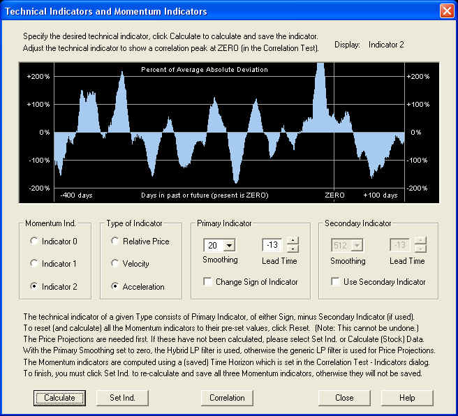
Technical Indicators Dialog
After opening the individual security data file, you will notice in the toolbar a button with a red "T" on it. When you click this button, the Technical Indicators dialog is shown:
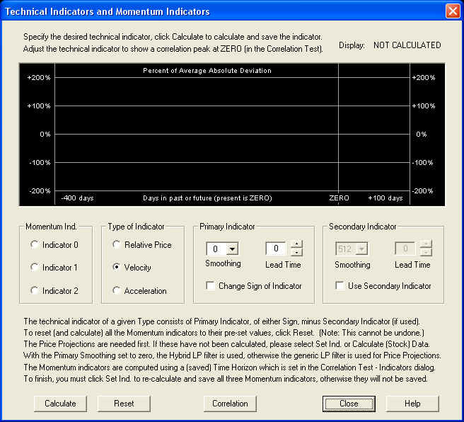
This is a rather complicated dialog, so we will show how it works here. Before you can test any technical indicators, you must first calculate a set of 1024 Price Projections. Normally you would do this by clicking the Calculate (Stock) Data button on the toolbar. This calculates the 1024 Price Projections, then calculates the Momentum indicators that are already saved (or for a new security file, the default indicators) and saves and displays these indicators in their respective splitter windows. Alternatively, if you want to reset the indicators to their default values, you can just open the Technical Indicators dialog as shown here and click the Reset button. This then resets all indicators to their default values and calculates them, using the Calculate (Stock) Data routine. The default values coincide with the Harmonic Oscillator indicators, with a quarter-cycle phase shift for the Relative Price and Acceleration indicators added, and no phase shift for the Velocity indicator.
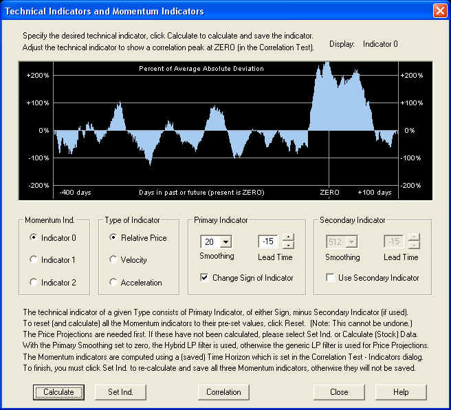
When the dialog first opens, the Relative Price, Velocity, and Acceleration indicators start with a Smoothing time scale setting of zero. This is a generic technical indicator, not one of the Momentum indicators, which can be tested just for experimental purposes. A Smoothing time scale setting of zero means that the Savitzky-Golay smoothing filter is not being used at all (except in the Secondary indicator of the Relative Price). With this setting, the Primary indicator of the Relative Price is just the (log) prices themselves, the Velocity indicator is just the returns, and the Acceleration indicator is the first difference of the returns. With the Smoothing time scale set to zero, the Hybrid Linear Prediction filter is used instead of the generic LP filter. So the Velocity indicator is just the output of the Price Projection (returns) itself. This is the setting shown above, which appears when the dialog is first opened. On the other hand, the Harmonic Oscillator indicator is obtained when the Smoothing time scale is set equal to the time horizon for trading. This is the default setting for the Smoothing time scale, which is set when the Reset button is clicked and the indicators (and Price Projection) is calculated. The default Lead Time for the Velocity indicator is zero, and that for the Relative Price and Acceleration indicators are the (minus) time horizon. This corresponds to a quarter cycle phase lead of these indicators. (The Relative Price is ahead of the Velocity by a quarter cycle in phase because the Change Sign of Indicator check box is checked.) Please note that the phases of these default indicators will not be correct unless the Correct Harmonic Oscillator Phase is done properly.
Relative Price Indicator
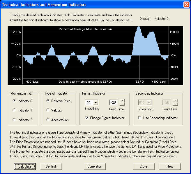
Starting with the Relative Price indicator, we can test the default indicator for correlation with future returns by first clicking the Calculate button to compute this correlation. The indicator is calculated and displayed in the window, and the result is the following:
Then click the Correlation button to call up the Correlation Test - Indicators dialog. We find:
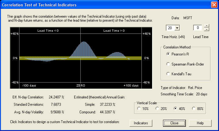
Since the Velocity indicator should be in phase with returns, we expect the Relative Price indicator to be a quarter cycle behind the Velocity. However, the Change Sign of Indicator check box is checked, so this sign-reversed Relative Price should be a quarter cycle ahead of the Velocity. With a Smoothing time scale of 20 days, a quarter cycle is roughly 20 days, so the Relative Price should be roughly 20 days behind the ZERO line. So when the Lead Time (in the Technical Indicators dialog) is set for -20 days, the Relative Price should be in phase with the returns, and the correlation peak should lie under the ZERO line. We see that the actual result is pretty close, although not exact. We can correct for this by shifting the phase so that the peak of the indicator is under the ZERO line:
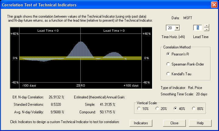
We see that the proper Lead Time adjustment is +5 days, leading to a 20-day correlation of almost 27%, and an excellent estimated annual gain (simple) of 41.31%. We can now switch back to the Technical Indicators dialog by clicking the Indicators button. To view the new Relative Price indicator, it is necessary to click Calculate again, since the Lead Time was changed. We find after this is done:
So after the adjustment, the overall Lead Time setting for maximum correlation with future returns is -15 days for the (sign reversed) Relative Price indicator. This seems to indicate that the effective window for smoothing for the Savitzky-Golay smoothing filter is actually a little less than twice the time horizon, where the window width should be roughly a half wavelength.
We have only adjusted the Lead Time control for maximum correlation with future returns. As can be seen, we could have also experimented with various settings of the Smoothing time scale for both of the components of this indicator (since it is a difference of two Relative Price smoothings), as well as different settings for the difference of the two Lead Time settings. (Notice that when we went from the Correlation Test - Indicators dialog back to the Technical Indicators dialog, the Lead Time setting was transferred to both the components of the indicator, thus preserving their difference.)
Velocity Indicator
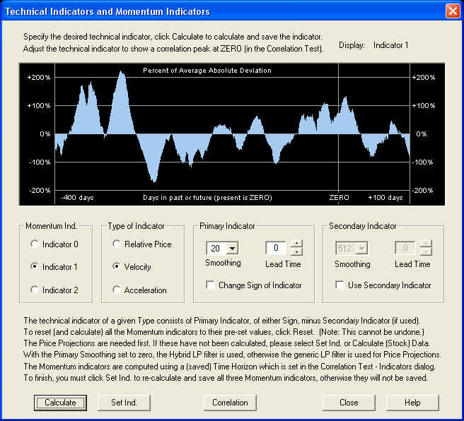
We now repeat the same analysis for the Velocity indicator. Selecting the default Velocity indicator and clicking the Calculate button to calculate it, we see the following:
Now clicking the Correlation button to bring up the Correlation Test - Indicators, yields the following result:
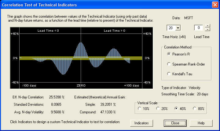
The Velocity indicator is exactly in phase with the future returns, and the correlation peak is centered exactly under the ZERO line. We would not expect anything less than this, since the above display is exactly the same as the one in the Correct Harmonic Oscillator Phase dialog, in which we manually set the phase or Lead Time so that the peak was exactly under the ZERO line as above. So everything is consistent.
Acceleration Indicator
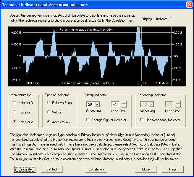
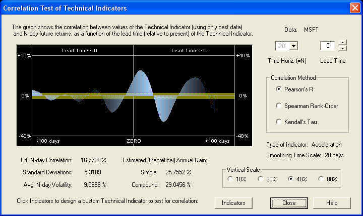
We now repeat the same analysis for the Acceleration indicator. Selecting Indicator 2 and clicking Calculate, the default Acceleration indicator appears in the Technical Indicators dialog as follows:
If we click Calculate to calculate the indicator, then click Correlation to call up the Correlation Test - Indicators dialog, we find:
We again find more or less the same result as with the Relative Price indicator, that this indicator is slightly out of phase, because a quarter cycle is a little less than 20 days. Adjusting the Lead Time control to bring the positive peak under the ZERO line, we find the result:
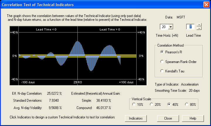
We find that the adjustment of the Lead Time in this case is +7 days, instead of +5 days as in the case of the Relative Price. Switching back to the Technical Indicators dialog by clicking Indicators, we may view the resulting indicator, after clicking Calculate again to re-calculate it:
The overall Lead Time of the Acceleration indicator is again -13 days instead of -20, indicating that the effective window for the smoothing filter is again a little less than twice the time horizon. Thus we now have a set of three compatible Momentum indicators, one of each type.
Now that all three Momentum indicators are specified and adjusted for maximum correlation with future returns, click the Set Ind. button to re-calculate and save all three indicators in the data file. Now the Technical Indicators dialog may be closed. If you want to work on the indicators some more, just re-open the dialog, since all three indicators along with the Price Projections are saved in memory as long as the security data file is open. The indicators themselves, but not the Price Projections, are saved in the security data file on disk.
Trading Rules Filtering
The Trading Rules consist of a weighted sum of the three Momentum indicators, with some additional "processing", or what we call filtering, performed. This is all accomplished within the Trading Rules Filtering & Momentum Weights dialog, which is displayed when the Trading Rules Filtering toolbar button is clicked. This is the green button with the purple letters "TR":
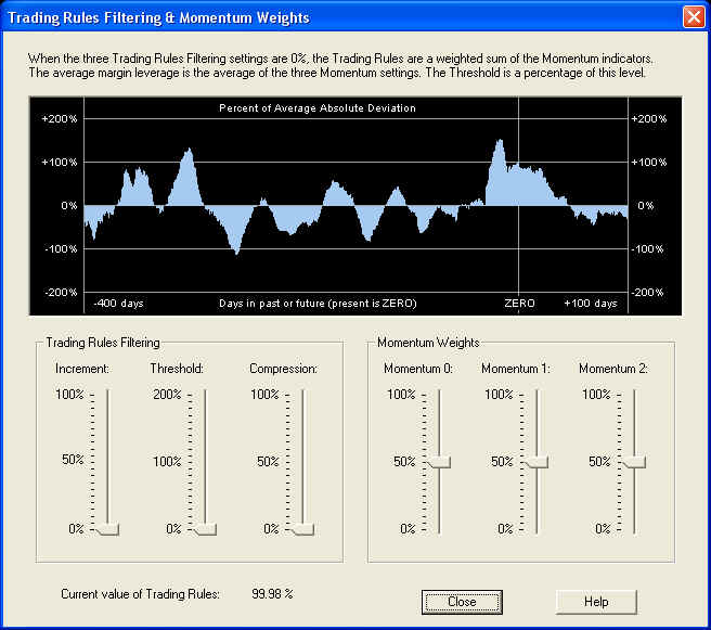
Displayed are the default settings, but the settings are saved in the data file, and the saved settings will appear when the dialog is called up. The three slider bars on the right control the Momentum Weights, which are the weights of the three Momentum indicators that make up the Trading Rules indicator. The indicator displayed in the graph above, with the three Trading Rules Filtering sliders on the left set to zero, is just this weighted sum of Momentum indicators. The three Trading Rules Filtering sliders control the size of the Increment, the level of the Threshold, and the amount of Compression of the Trading Rules. You can experiment with these three controls to see exactly what they do. For example, with each control set to its mid-range, the result is as follows:
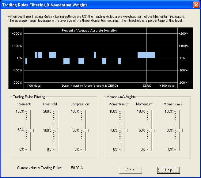
The relevant quantity is the value of the Trading Rules at the present time, which is the value under the ZERO line. This value is displayed at the bottom of the dialog for convenience, so if you want to check this you can just open this dialog. This is the value which gives the recommended trading position for the next N days, where N is the time horizon. The Trading Rules are computed from the saved Momentum indicators, so it is not necessary to run Calculate (Stock) Data to display them. The new Trading Rules are computed and displayed in the graph window each time one of the slider bars is moved, and the settings for all six sliders is saved in the security data file. This same dialog box is also used in the Diagnostic Test to select temporary settings for testing. I that case the settings are only used for the test and are not saved.
Conclusion
Here is a view of the three Momentum indicators in their splitter window:
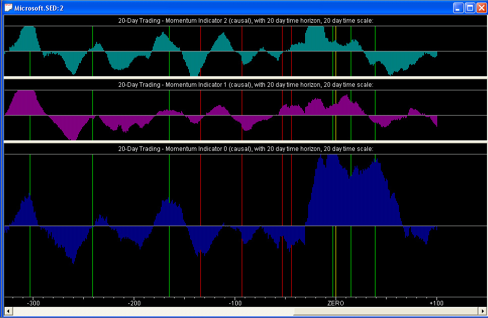
It is rather pleasing to see how all three Momentum indicators line up (approximately) with each other. We also know that they line up with the returns on the 20-day time horizon, since we have specifically adjusted the indicators for maximum correlation with future returns on this time horizon. The Weighted Sum of Momentum Indicators on the Forward MA indicators splitter window should therefore line up with the 20-day forward MA of the returns, since the correlation has been maximized between the Momentum indicators (on the 20-day time horizon) and the returns over a 20-day time horizon.
Now we may verify the measured correlation by running the Diagnostic Test. Clicking the Diagnostic Test button on the toolbar brings up the Trading Rules Filter & Momentum Weights dialog again. If we select the default settings and then click Proceed, the Diagnostic Test dialog then appears with a list of the settings:
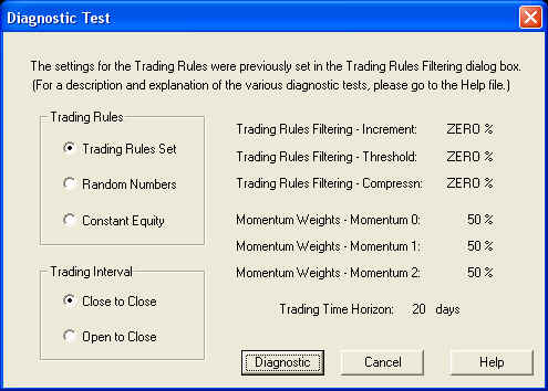
Clicking Diagnostic then causes the Diagnostic Test to run. This test depends only on the saved Momentum indicators, so it is not necessary to run Calculate (Stock) Data to run this test.
The results of the Diagnostic Test are expressed in terms of simple annual gain, corrected for 100% margin. For comparison with the results of the Correlation Test given above, we note here the estimated (theoretical) simple annual gain, from the dialog boxes shown previously, for each of the three indicators:
Momentum 0: 41.31% Momentum 1: 47.13% Momentum 2: 46.01%
|
Test |
Mom. 0 |
Mom. 1 |
Mom. 2 |
Mix. |
|
TR Set |
31.35% |
25.64% |
26.43% |
32.05% |
By contrast, the Buy & Hold return was -3.91% over the time interval. Considering the rather large statistical variance of the results of active trading, the measured gains agree acceptably well with the estimated gains, although for some reason they are all somewhat too low.
Of course, these are only simulated results. Although every effort has been made to make this a valid and fair test of the predictive capability of the Momentum indicators, there is no way to say with certainty that no future knowledge has crept in somewhere. The Diagnostic Test is only an estimate or simulation of various trading scenarios, not the real thing. QuanTek makes use only of past price data to derive the Price Projection and Trading Rules, not fundamental or economic data. In real-life trading or investing, the trader or investor must make use of all available information in formulating trading and investing decisions.
return to Demonstrations page