Demo: Periodogram and Wavelet Spectrum
(Revised June 27, 2006)
According to the theory of stationary stochastic time series, the properties of the time series are described by the mean and the autocovariance sequence, which are constant in time since the series is stationary. The time series in question here is the series of returns, or daily (logarithmic) price changes. In the classical Random Walk model of stock prices, the returns series is just Gaussian white noise, which means that the correlation between any two different days of returns is zero, and the mean and variance are constant. However, this is known to be only a crude approximation for financial time series. So the goal is to find small departures from randomness, or in other words correlation, in the returns series, and to exploit this correlation to construct profitable Trading Rules.
For a stationary time series, the autocovariance sequence is uniquely determined by the power spectrum and vice-versa. This is called the Wiener-Khinchin theorem -- the two are the Fourier transform of each other. From the autocovariance sequence or the power spectrum it is then possible to compute the coefficients of a Linear Prediction filter, to compute the best estimate of the future returns of the price series, or in other words a Price Projection. If the Random Walk model holds, then the autocovariance sequence is zero for time lags greater than zero and is just the (constant) variance for zero time lag. (The constant mean of the returns is just the constant trend of the Random Walk.) The corresponding power spectrum is a constant -- white noise. If there is any departure from a constant power spectrum, this indicates the presence of correlation in the time series, and hence the possibility of making a partial prediction or estimate of the future returns. (Note: The correlation of two quantities is the covariance divided by the standard deviation of the two quantities.) For financial time series, since we are only working with daily returns, it is reasonable to assume that the data are stationary over a period of 1024 days -- about 4 years. Then we can utilize the theory of stationary time series as a reasonable approximation to the actual non-stationary financial time series.
Periodogram Spectrum -- AAPL
For a representative Periodogram power spectrum, we can consider the case of AAPL stock. Here is the Periodogram display for this stock:
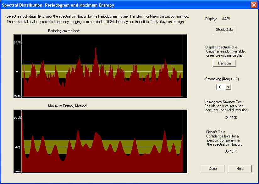
The top pane is the standard Periodogram, as described in most textbooks on Time Series Analysis. The horizontal axis represents frequency, corresponding to a period of 1024 days on the left side to 2 days on the right. The middle of the graph corresponds to a period of 4 days, half the maximum (Nyquist) frequency. So the entire right half of the graph corresponds to periods of 4 trading days or less. This half of the graph is probably just stochastic noise, and that is certainly the way it appears in this graph. Clicking on the Random button, you can compare the graph to one generated from Gaussian random numbers, and there is not much difference at first glance. According to the standard theory, each frequency component of the Periodogram is a random variable with a standard deviation of 100% -- completely random. The only way to get a meaningful result, therefore, is by smoothing the Periodogram. You can set the smoothing time period to a wide range of values -- here it is set to 6 days. In the present case, however, the spectrum appears random, for any smoothing, and this is verified by the Kolmogorov- Smirnov test, which compares the cumulative spectrum to a straight line and measures the maximum deviation. Since most of the spectrum is high-frequency in nature, we must conclude that this high-frequency spectrum is essentially stochastic noise.
However, notice the very low frequency end of the power spectrum. This shows a distinctive spike at the lowest frequencies, corresponding to a long-term trend. This is just the kind of behavior that is expected from the power spectrum of a fractionally differenced stochastic process, obeying fractal statistics. People like Benoit Mandelbrot (the "inventor" of fractals) and Edgar Peters have written about this, postulating that financial time series are actually of this type. This would also agree with the idea of trend persistence, which is an important principle of Technical Analysis. The idea is that the long-term trend that existed in the past should persist into the future, or that there is a positive correlation between the long-term trend in the past and that in the future. In other words, the low-frequency components of the spectrum should display a positive correlation, and that in turn means that the spectrum should display a positive "spike" at low frequencies (according to the standard theory of a stationary stochastic process). So it is just this kind of positive spike at low frequencies that we want to see if there is to be trend persistence and correlation between low-frequency technical indicators based on past data, with future returns.
From the Periodogram spectrum, it is possible to calculate directly the coefficients of a Linear Prediction filter, and some of the filters used by QuanTek use this technique. On the other hand, the LP coefficients can be calculated by a different method, and then the spectrum computed from these LP coefficients. This method of computing the spectrum is called the Maximum Entropy method, and is displayed in the bottom pane of the dialog box. By comparing the two, you can see that they agree rather closely, up to the degree of smoothing of each. (You can view both displays with no smoothing at all, by setting the Smoothing to 1 day.)
Wavelet Spectrum -- AAPL
Another way to compute the power spectrum is to use the Discrete Wavelet Transform (DWT) instead of the Discrete Fourier Transform (DFT) -- otherwise known as the Fast Fourier Transform (FFT). The Fourier Transform decomposes the signal using a basis of "infinite" sine waves of a single precise frequency. The Wavelet Transform, on the other hand, uses a basis consisting of localized (in time) "wave packets" which are of finite extent in both the time and frequency domains. Thus the Wavelet decomposition of the signal has coefficients that depend on both the frequency (octave) as well as time, as opposed to the Fourier decomposition whose coefficients depend only on frequency.
For a representative Wavelet power spectrum, consider once again the case of AAPL stock:
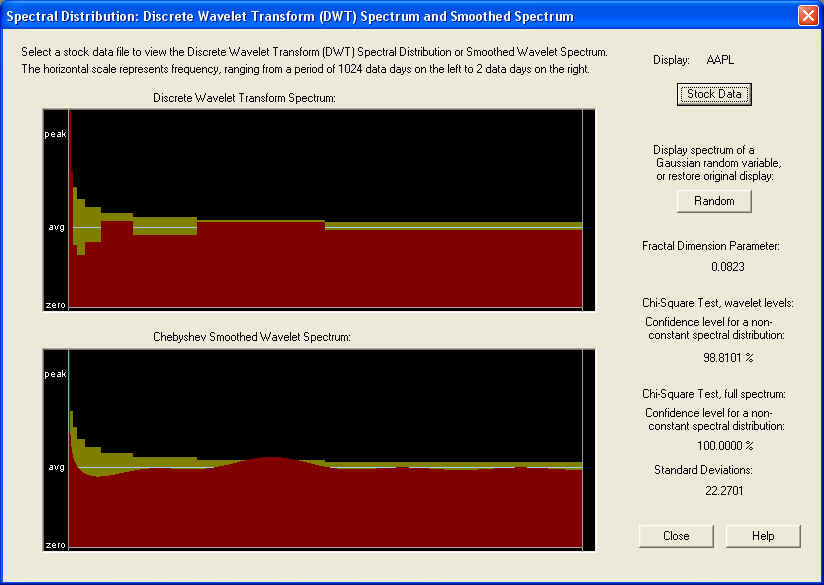
The upper graph shows the DWT power spectrum (the square of the DWT coefficients), which have been averaged within each octave over all time values. Before this averaging is done, there are 512 DWT coefficients, the same number as for the DFT, but after the time averaging there are only 9 values of the power spectrum, one for each frequency octave. These octaves can be seen above, in which the frequency range has been split into regions which differ from the previous region by a factor of two (an octave). The lower graph shows the same spectrum, which has been smoothed using Chebyshev polynomials, for use in the Wavelet Linear Prediction filters. (Note: The yellow band represents the one-standard-error bars for each frequency octave. The band is wider for the lower frequency octaves because there are fewer DWT components in these octaves.)
For a statistical test of randomness, a Chi-Square test was adopted. In the above example, the spectrum appears completely random according to this test. This may be due to the fact that after the time average is taken, there are only 9 components of the power spectrum left. However, when the Chi-Square test is performed on the full 512 time-dependent components of the DWT spectrum, the test gives an amazing 22+ standard deviations away from a random result. This may be due to correlation in the spectrum, which is averaged out when the time average is taken, or perhaps due to the fact that the distribution of the returns is non-Gaussian, or perhaps both. But this result, which is consistent for all stocks, implies that perhaps an adaptive filter based on non-stationary time-dependent statistics could be developed, based on this Wavelet decomposition. We are still working on this problem.
As in the case of the Periodogram, the low-frequency spike is clearly visible in the Wavelet spectrum. In fact, the main goal in adopting Wavelets was to display this low-frequency behavior more clearly. This particular case would provide evidence for fractal statistics with long-memory, or in other words a fractionally differenced process with positive fractional difference (or fractal dimension) parameter. Notice that the measured fractal dimension in this case is positive, approximately +0.08. The positive spike in the lowest frequency octaves implies that there should be a positive correlation between the long-term trend and future long-term returns. This correlation, although small, can lead to significant gains if properly utilized in an appropriate set of Trading Rules.
Periodogram Spectrum -- MSFT
By way of contrast, let us now look at the Periodogram for MSFT stock:
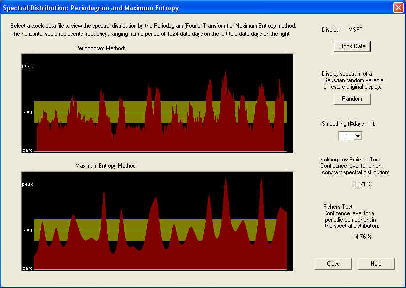
According to the Kolmogorov-Smirnov test, the confidence level for a non-random spectrum is a respectable 99.71%, much higher than for AAPL stock. Looking at the graphs, it appears that the power spectrum is concentrated more in the second half of the frequency range, corresponding to periods from about 5 days down to 2 days. So maybe there is a certain amount of predictability in the short-term trading rules for this stock. There is another concentration of spectral power about a quarter of the way from the low-frequency end, which would correspond to about a two week period. However, a major difference from the case of AAPL is that, in this case, there is no sharp peak at the very low frequency end. Instead we see a pronounced dip at this end. When the spectral power starts with a low value at the low frequency end and then rises with increasing frequency, this indicates anti-correlation between past returns and future returns. So if the stock went up in the past, it is more likely than not to go down in the future, and vice-versa. In other words, what we have is a return to the mean mechanism for this stock. This is confirmed by looking at the graph of MSFT, which appears very flat going back a couple of years at least. Another way to put it is that MSFT is not in a trend mode, but rather appears to be in a trading range.
Wavelet Spectrum -- MSFT
This is seen more clearly by looking at the Wavelet Spectrum for this stock:
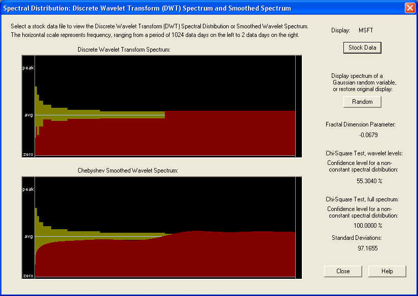
From the DWT spectrum, it is very clear that the spectral power at the lowest frequencies is deficient, and rises with increasing frequency. This is just the kind of behavior that is expected from a fractionally differenced process with negative fractional difference (or fractal dimension) parameter. And indeed, that is the result of calculating this parameter, as shown. This kind of spectrum seems to be typical at the present point in time, which seems to indicate that the overall market is in a return to the mean mode or trading range. Back in the late '90s the market was in a trend mode, and in this case most stocks would have probably displayed a pronounced peak at the low frequency end, and a positive fractional difference (or fractal dimension) parameter. This is probably the basis of the claims that have been made that this is the generic condition for the market, but more probably the fractional difference parameter changes with time, as the market moves from a trending to a trading market, and back again.
As in the case of AAPL, the Chi-Square test for the 9 time-averaged Wavelet spectrum octaves does not indicate a significant departure from randomness, but the Chi-Square test for the full set of 512 Wavelet spectrum components does show an amazing 97+ standard deviations away from randomness. Once again, this is either due to correlation that is averaged over in the time average, or the fact that the distribution of returns is non-Gaussian, or both. This once again seems to indicate non-stationary statistics, so maybe this could be utilized to advantage in an Adaptive Wavelet Linear Prediction filter.
Higher-Order Statistics
The Periodogram Spectrum and Wavelet Spectrum measure the power spectrum of the auto-correlation sequence of the (logarithmic) price returns. These correlations, or more precisely the covariance and variance, together with the mean of the returns, idealized as a stationary stochastic process, constitute second-order statistics of this stationary process. It is thought that at the second-order level, the returns are essentially uncorrelated white noise, but we are finding some significant correlation after filtering out the high-frequency components, leaving only the low-frequency components. From the above displays, it can be seen that the high-frequency components constitute most of the power spectrum, which explains why the low-frequency correlation is so easily masked by the high-frequency stochastic noise. Of course, there may be (time-dependent) correlation in the high-frequency components as well, but our idealization that the process is stationary over a period of 1024 days is unable to find this high-frequency correlation. This is why an Adaptive Wavelet Linear Prediction filter would be desirable.
However, there is also the possibility of higher-order statistics. It is known already that there is significant autocorrelation in the sequence of daily volatility (absolute value of the returns) and in the squares of the returns. These are non-linear functions of the returns, and to make a projection of these quantities requires non-linear filtering techniques. But these higher-order auto-correlations and auto-covariances can be described by their power spectrum just as in the case of second-order auto-correlation, and in the case of the cross-covariance, the corresponding spectrum is called the cross-spectrum. So similar, though more complex, filtering techniques can be used to project these higher-order correlations as are used in the second-order case. In general, several of these sequences would be projected at once using multivariate prediction filters, rather than the simpler univariate prediction filters used for the basic Price Projection. Once again, the absence of correlation would be indicated by a flat power spectrum (white noise), while correlation would show up as a non-flat power spectrum. The filter coefficients could once again be derived from these power spectra, at least in the stationary case.
Utilizing higher-order statistics would provide the connection between Signal Processing and traditional Technical Analysis. The whole objective of Technical Analysis is to find complicated functions of past price data, which are supposed to be correlated with future returns. Some of the indicators of traditional Technical Analysis are highly complex patterns or functions of the past price history, and highly nonlinear functions. So these complex technical indicators would utilize higher-order statistics of a very high order! The problem with this is that the higher the order, the more cross-spectra there are to estimate, and there is only a limited amount of data in most financial time series. So to actually measure statistically the effectiveness of such complex patterns of such high order is virtually impossible. So this is a good reason to focus attention on second-order statistics and maybe fourth-order statistics, and construct simple oscillator-type technical indicators based upon these.
return to Demonstrations page