Demo: Trend Persistence and Smoothness
(Revised May 26, 2005)
One fundamental premise of the QuanTek approach is that some correlation exists in the stock data in the low-frequency modes. In other words, if the stock returns data are separated into separate frequencies by means of the Fourier transform, then the low-frequency modes exhibit some persistence, while the high frequency modes are essentially stochastic noise. (This idea may need to be modified by the observation of some anti-persistence of stock returns at the day-trading scale, for some stocks.) Nevertheless, the concept of trend persistence is very solidly entrenched in financial trading. This idea can be realized by supposing that the true "signal" consists of the lower frequency modes, and by virtue of being low frequency, this signal can be regarded as smooth. (This means, technically, that all of its derivatives up to a very high order are continuous.) This is to be contrasted with stochastic white noise, which is discontinuous everywhere and has no derivatives. White noise is defined as having a spectrum which is constant, from the lowest to the highest frequencies. But if the signal, consisting of lower frequencies only, is superimposed on white noise, then the signal can theoretically be isolated by smoothing the data and removing the higher frequencies, leaving only the smooth signal and some lower-frequency noise components. We will investigate how this idea works in an ideal, artificial case in which the signal is a pure sine wave of low frequency, with some stochastic noise added. (We created this file by starting with the S & P 500 returns data and adding a low frequency sine wave of large amplitude.) We then observe the appearance of the various QuanTek displays and indicators with this idealized data.
Price Projection Filters
The original version of the QuanTek program, which was called StockEval, used a Linear Prediction filter for the Price Projection and Trading Rules. This filter was a standard filter, published in the public domain, which can be found in Numerical Recipes (1992). There is (at least) one major difference between this filter and the Fractal Difference filter used in QuanTek, which can be found in Time Series: Theory and Methods, (1991). They both apply to stationary processes, but the Fractal Difference filter is fixed except for one adjustable parameter, the Fractional Exponent (or Dimension). The Linear Prediction filter, on the other hand, has many adjustable parameters, which are adjusted by means of an estimation procedure. If the data set is N units long, in fact, the maximum number of adjustable LP parameters in the filter is N-1. Normally, the filter is used with only a small number of LP parameters, which means that the parameters are fit to small data segments and use only small data segments for prediction. To use the entire N-1 parameters for a fit to the data enables the whole data set to be used for prediction. This, in turn, enables us to capture the low-frequency, long-wavelengths modes and correlations in the data. However, it also means that, in essence, the filter coefficients are a perfect fit to the noise. This problem is then solved by using the Savitzky-Golay smoothing filter to eliminate the high-frequency modes, effectively eliminating most of the LP parameters and reducing the action of the filter to these low-frequency modes only. This approach seemed to work well in the trending market of the late '90s, which exhibited a lot of trend persistence.
Here is the TEST data file using the Linear Prediction for the Price Projection (the blue part to the right):
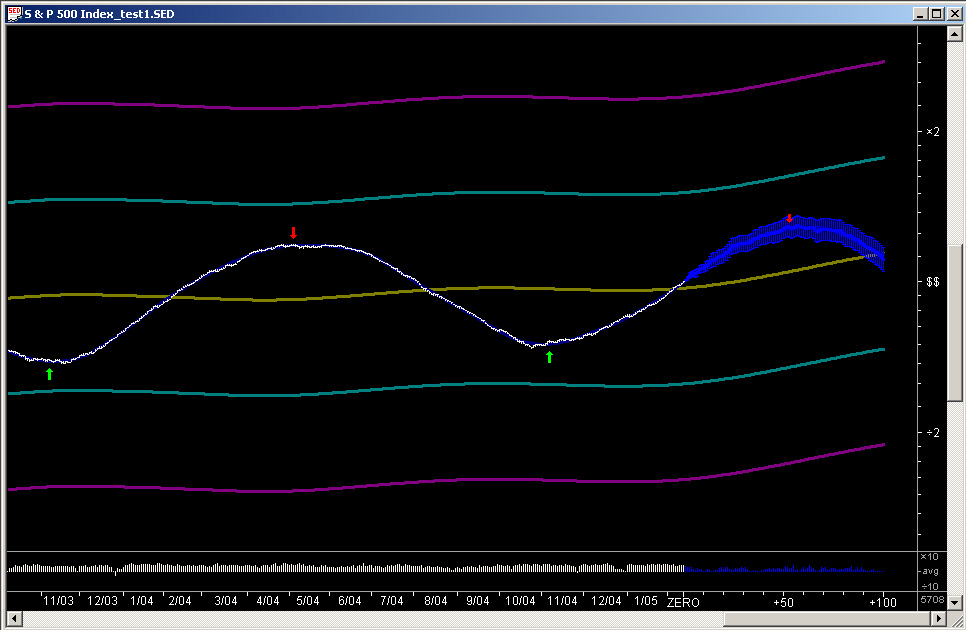
As can be seen,, the Linear Prediction routine projects the smooth sine wave quite well. This is not too surprising, since the sine wave (with added noise) is very smooth and highly auto-correlated. It is the main forte of the Linear Prediction filter that it performs well on very smooth, but not necessarily exactly periodic, waveforms.
Here is the TEST data file using the Fractional Difference filter with a fractional exponent of +0.25 for the Price Projection (the blue part to the right):
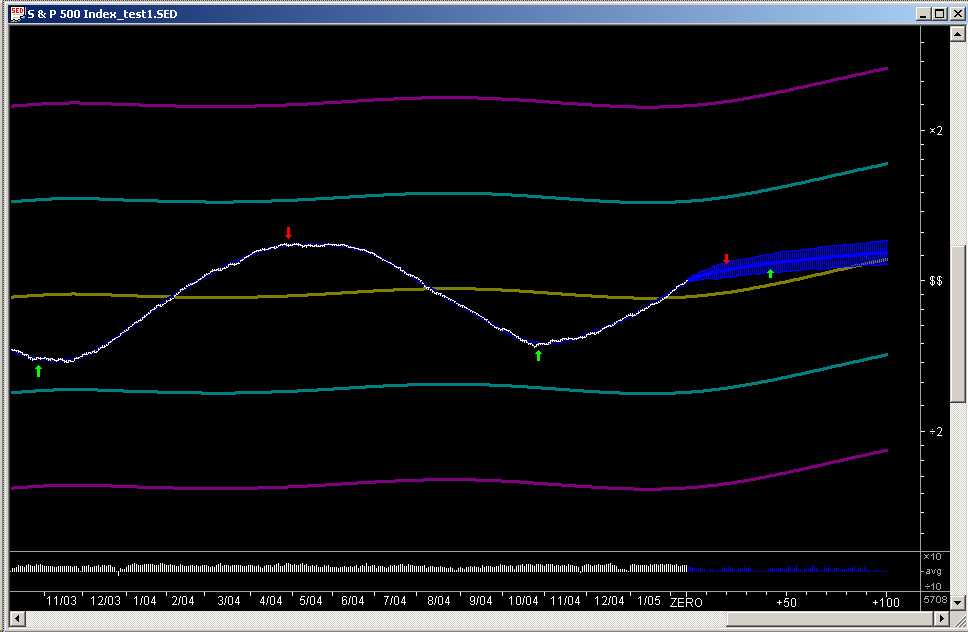
Note that this filter is set for a positive fractional exponent, so it should capture the trend persistence of the smooth curve. Nevertheless, for this smooth sine wave, the Fractional Difference filter does not perform as well as the Linear Prediction filter.
Here is the TEST data file using the Fractional Difference filter with a fractional exponent of -0.25 for the Price Projection (the blue part to the right):
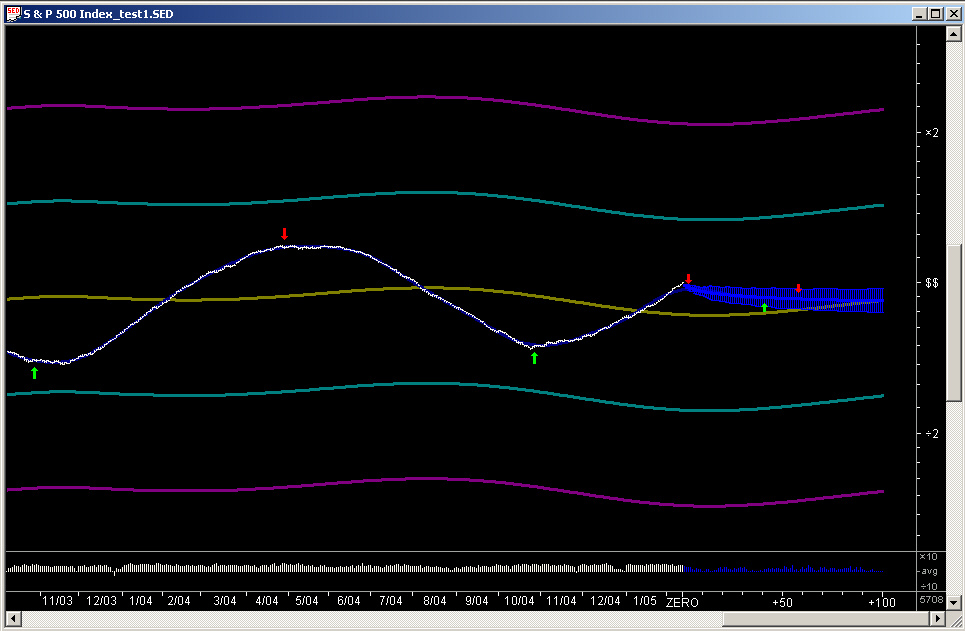
Note that this filter is set for a negative fractional exponent, so it should capture any anti-persistence of the data. Thus it can be seen that this anti-persistent filter is completely wrong for projecting this smooth sine wave. On the other hand, this filter works well for some stocks in the present time era which seem to exhibit a strong short-term anti-persistence of the returns, such as MSFT over the past four year or so.
(Note in the above graphs that the dark yellow 320-day smoothing curve from the Savitzky-Golay smoothing filter, seems to be out of phase with the signal. However, this is merely a consequence of the fact that the smoothing time period is something of the order of 3 half-wavelengths of the sine wave.)
It appears that the appropriate projection filter to use depends on the individual stock and also on the time period in question. At the current time, some stocks are displaying a rather strong anti-persistence in the short-term returns, so the Fractional Difference filter with negative fractional exponent gives the best results. At other times, such as in the trending market of the '90s, perhaps the Fractional Difference filter with positive fractional exponent gives the best results, or perhaps the Linear Prediction filter works the best. The stock data, of course, are very noisy and at times anti-persistent, unlike the smooth sine wave, so it should not be inferred that the Linear Prediction filter will work best for stock returns data, just because it leads to the best projection of the smooth sine wave. It becomes evident at this point that perhaps the appropriate solution would be a combination ARIMA (Auto-Regressive Integrated Moving Average) filter, combining the low-frequency persistence with the high-frequency anti-persistence, with only a few parameters to estimate. It is the over-estimation with far too many filter parameters that is the main weakness of the Linear Prediction filter, along with its inability to simulate a fractionally integrated (the "I" in ARIMA) process. In fact, the Linear Prediction filter simulates Auto-Regressive processes only (the "AR" in ARIMA).
One might also consider the possibility of some sort of Adaptive filter, such as the Kalman filter. The problem here is that the financial data are probably too sparse to be able to segment the data and detect a changing correlation structure in each segment (except maybe for the short-term correlation). So for the practical reason of not enough data points, it is necessary to treat the data as if it were stationary and compute correlation over the whole data set, or at least over only a few large blocks of data. Stationarity, of course, is a key assumption of the ARIMA class of processes.
Technical Indicators
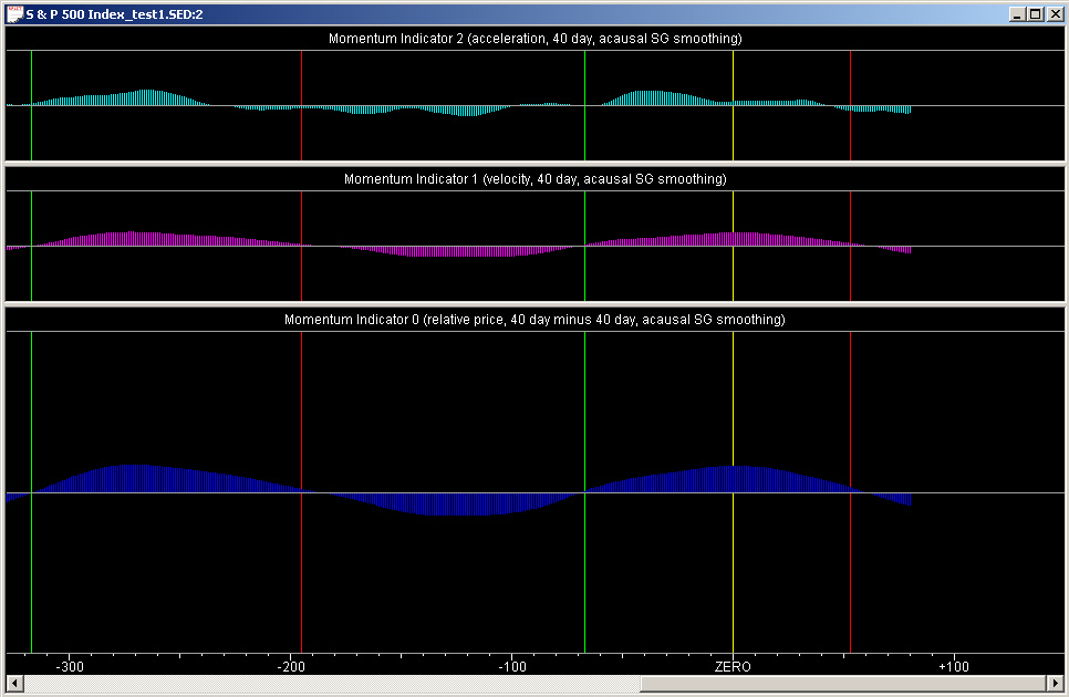
We now confine our attention to the results using the Linear Prediction filter, as shown above. We examine to begin with, the first group of QuanTek technical indicators, consisting of three indicators in the Harmonic Oscillator splitter window. These consist simply of the Relative Price (bottom pane), Velocity (middle pane), and Acceleration (top pane), which are 40-day smoothings of the data from the Savitzky-Golay smoothing filter, with no derivative, 1st derivative, and 2nd derivative, respectively:
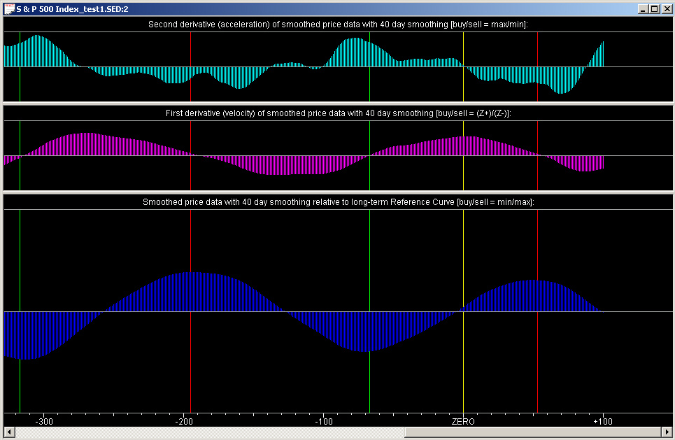
The Relative Price and Velocity indicators show mainly the pure sine wave only, while the Acceleration indicator is starting to show the acceleration due to the superimposed S & P 500 data as well. The green and red lines are the buy/sell points derived from the Trading Rules indicator (discussed later). The yellow line is the present day (day ZERO), and all data to the right of the ZERO line are due to the Price Projection. Notice the relative phases of the three graphs. The buy/sell points correspond to a Relative Price which is minimum/maximum (min/max) (relative to the 320-day smoothing curve), to positive/negative zero crossings (Z+/Z-) of the Velocity curve, and to the maximum/minimum (max/min) of the Acceleration curve. Notice that these points line up rather well, even though they are derived from the Trading Rules indicator, which is derived somewhat differently. This is crucially dependent, however, on all indicators using the same type of smoothing, namely the Savitzky-Golay (acausal) smoothing filter with the same time scale.
To re-iterate, the buy points are when the price is minimum, the velocity (returns) are going from negative to positive, and the acceleration (curvature) is at a positive maximum. These points correspond to a trough or minimum point of the prices. The sell points are when the price is maximum, the velocity (returns) are going from positive to negative, and the acceleration (curvature) is at a negative minimum. These points correspond to a peak or maximum of the prices. Also notice that these buy/sell points correspond to the green/red arrows in the price graph shown above (using the Linear Prediction filter). These indicators in the Harmonic Oscillator splitter window are independent of the custom Momentum indicators and Trading Rules, except for the indicated buy/sell points. They serve to confirm these latter indicators.
Relative Price Indicator
We begin by trying to design a custom Technical Indicator which is a generic Relative Price indicator. We start with the following settings on the Technical Indicators dialog:
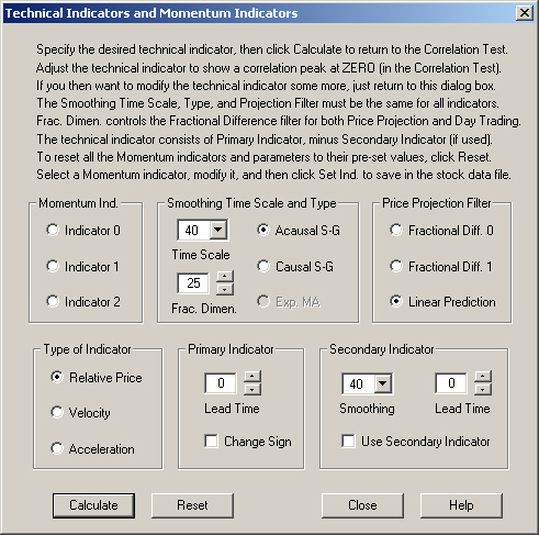
This indicator has zero Lead Time and uses only the Primary Indicator. Calculating the correlation with 1-day returns leads to the following result:
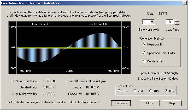
This is the kind of result we expect. The correlation is very large at the peaks, of course, because the signal is an almost perfectly deterministic sine wave. But we expect that the higher the price in the past, at a time in the past about a quarter of the cycle, the more negative the future 1-day return. The lower the price a quarter cycle in the past, the more positive the future 1-day return. In other words, there should be a negative correlation between past prices and the future 1-day return, which peaks at about a quarter cycle in the past. This is indeed what we see in the graph. The correlation between the present price, at the ZERO line, and the future 1-day return, is nearly zero, because the price cycle is one quarter cycle out of phase with the returns cycle. Likewise, the return 1-day in the future is positively correlated with the price one quarter cycle in the future, because the price in the future is a direct consequence of the rate of change of prices at the present.
To turn this into a Technical Indicator, we must shift the phase. Let us try an indicator consisting of a positive contribution of the Relative Price at a future time, and a negative contribution of the Relative Price at a past time. Thus we try the following settings:
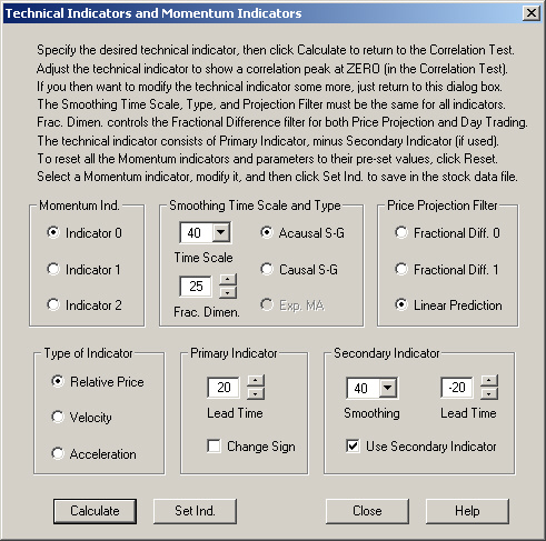
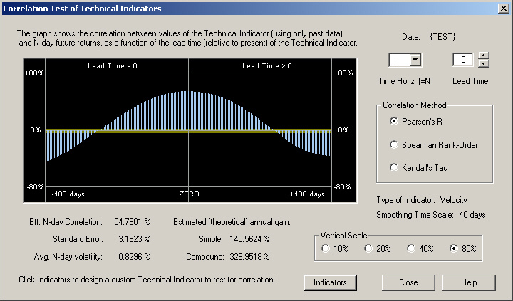
The Use Secondary Indicator check box has been checked, and the Lead Time for the Primary Indicator has been set to +20 days, while the Lead Time for the Secondary Indicator has been set to -20 days. This leads to the following correlation with 1-day returns:

Now we see that the resulting Technical Indicator is nicely peaked near the ZERO point in the graph. The actual value of the Correlation and Estimated annual gain should be ignored, since, of course, we are working with a nearly perfectly deterministic sine wave. But this illustrates the ideal behavior that a good Technical Indicator should display. This indicator is a function of past prices which exhibits a strong positive correlation with future 1-day returns.
Velocity Indicator
We now try to construct a Technical Indicator of the Velocity type. In other words, this will be a function of the past returns, or first derivative of the past prices. We start with the following generic settings in the Technical Indicators dialog:

Upon computing the correlation of the smoothed past and future projected returns with the future 1-day returns, we find the following result:
This result is as we expect. The smoothed returns of the deterministic sine wave signal are at maximum correlation with the future 1-day returns near the ZERO point (actually one day in the future of it). Thus we have another valid Technical Indicator, which this time is a smoothed function of the past returns or first derivative of prices, which is strongly correlated with the future 1-day returns.
Acceleration Indicator
Now let us try to construct a generic Technical Indicator of the Acceleration type. This will be a smoothed function of the second derivative of past prices, which is the same thing as the rate of change of returns. We start with the following generic settings in the Technical Indicators dialog:
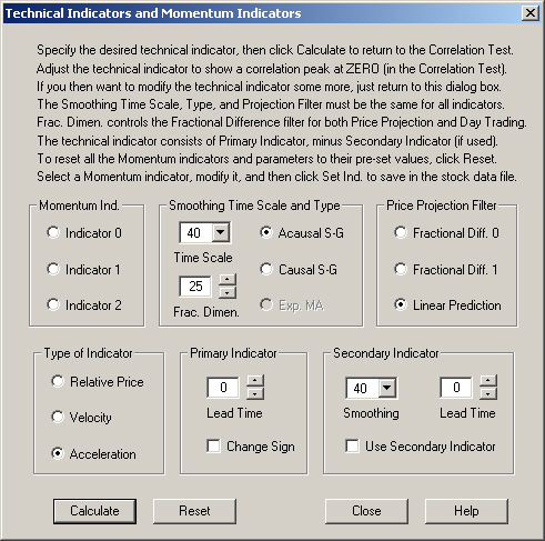
This leads to the following correlation of the smoothed second difference of past prices with future 1-day returns:
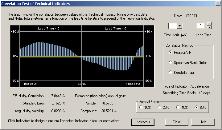
This graph is also what we expect for the correlation of the past acceleration with the future 1-day returns. When the past acceleration is positive, indicating an upward curvature of the prices or increase in returns, this will lead to a positive future 1-day return. Likewise, when the past acceleration is negative, indicating a downward curvature of the prices or decrease in returns, this will lead to a negative future 1-day return. In the future, due to the cyclic nature of the price graph, a positive future 1-day return will lead to a negative acceleration or downward curvature in the future, and a negative future 1-day return will lead to a positive acceleration or upward curvature in the future. So this is the kind of graph we expect of the correlation of past acceleration with future 1-day returns, given that the price "signal" has low-frequency correlation.
To construct an actual technical indicator, we need to shift the phase. Let us simply take the acceleration some time in the past as our technical indicator. The settings in the Technical Indicators dialog then become the following:
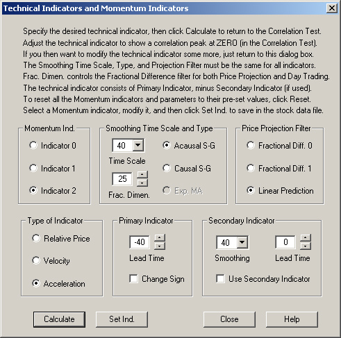
This then leads to the following correlation between this technical indicator and the future 1-day returns:
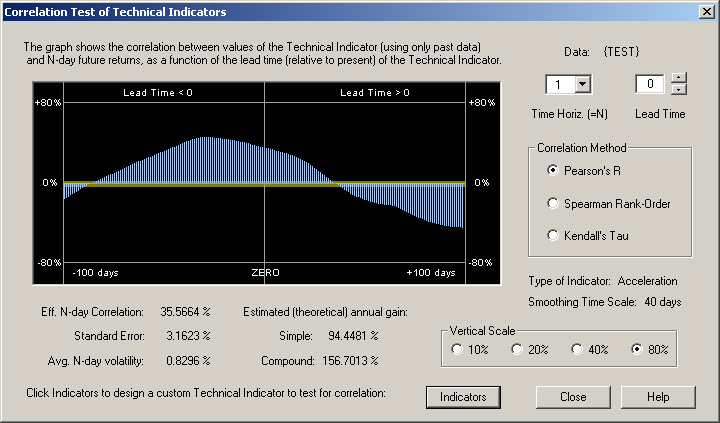
For this indicator, in which the Lead Time is set to -40 days, we arrive at a good positive correlation between this technical indicator and the future 1-day returns. However, it can be seen that the correlation would be even better if we had gone further back into the past.
Momentum Indicators
Now we can view the Momentum Indicators splitter window, which shows all three of the above technical indicators, after they have been saved as the respective three momentum indicators:
(Note that the normalization of these indicators seems to be a little off due to the predominance of a single sine wave in the signal.) The important point to note here is that the peaks, troughs, and zero crossings of all three of the indicators line up pretty well. (Again, the Acceleration indicator is a little non-regular due to the influence of the S & P 500 data on top of the sine wave.) The buy/sell points correspond to the positive/negative zero crossings of the indicators. Therefore it can be seen that the momentum indicators behave the same way as a velocity. The momentum indicators are to be interpreted as a surrogate or estimate for the (smoothed) returns, both past and future, and the smoothed returns are the same thing as the velocity.
These three momentum indicators are to be added together to form the Trading Rules indicator. You can set the relative weight of each of the three indicators by means of the Trading Rules Parameters dialog box:
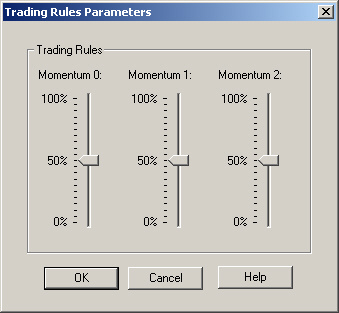
In the present case, all three momentum indicators are given equal weight in the Trading Rules indicator.
Trading Rules Indicator
Now we may see the result of combining these three momentum indicators to form the Trading Rules indicator. This indicator is in the bottom pane of the Trading Rules splitter window:
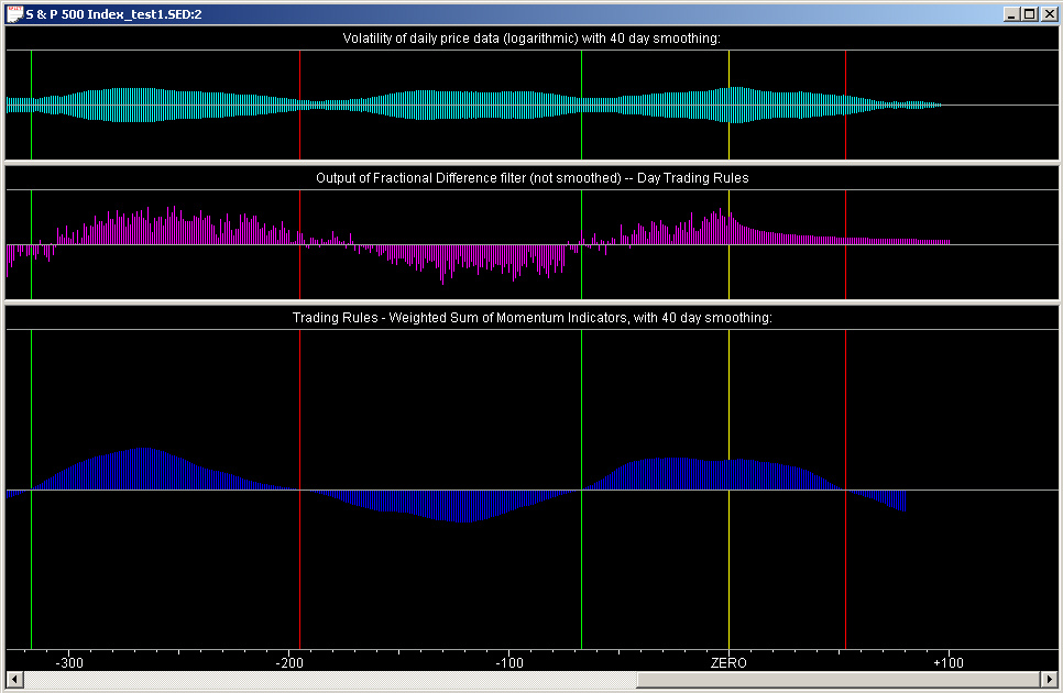
The positions of the buy/sell points are determined from the positive/negative zero crossings of this indicator. As before, these are denoted by the green/red vertical lines.
The middle pane of this splitter window is the output of the Fractional Difference filter, which is used for the Day Trading rules. This graph is the only one that is not smoothed. It is computed by going back and computing the 1-day expected return from the Fractional Difference filter for each day in the past, using only data before that day. In this way it is actually a causal display, unlike all the other graphs which are acausal, being the output of the acausal Savitzky-Golay smoothing filter. But it can be seen that, for the given sine wave signal, the output of the Fractional Difference filter corresponds nicely with the past part of the smoothed momentum indicator, which is calculated in a completely different way (using the Linear Prediction filter as explained previously).
As a matter of fact, we can test the output of the Fractional Difference filter itself in the present case. We use the following settings on the Technical Indicators dialog to test the (unsmoothed) output of the Fractional Difference filter as a technical indicator (with a Smoothing Time Scale of 1 day corresponding to no smoothing). Note that the Fractional Dimension (exponent) is set to a positive value of +0.25, indicating trend persistence:

This then leads to the following correlation with the actual 1-day future returns in the Correlation Test dialog:
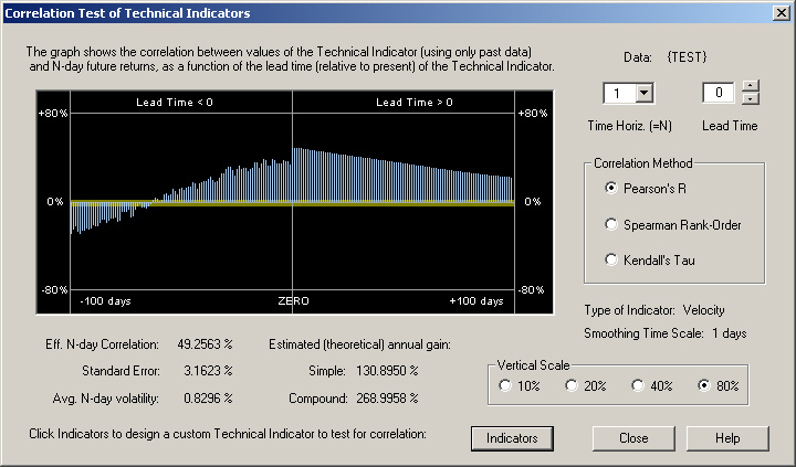
Here we see that, due to the (extremely!) persistent trend of the sine wave, the past returns are highly correlated with the future 1-day return, and the output of the Fractional Difference filter is even more highly correlated. This positive correlation is also very visible in the middle pane of the Trading Rules splitter window.
Finally, the upper pane of this splitter window shows the Volatility of the data. It can be seen that the buy/sell points tend to pass through the areas where the volatility is at a minimum. The natural explanation for this is that the buy/sell points occur at the peaks and troughs of the price graph, where the volatility is minimized due to the fact that the price trend is zero at these points.
Periodogram
Finally, we can take a look at the Periodogram or spectrum of this pure sine wave signal:
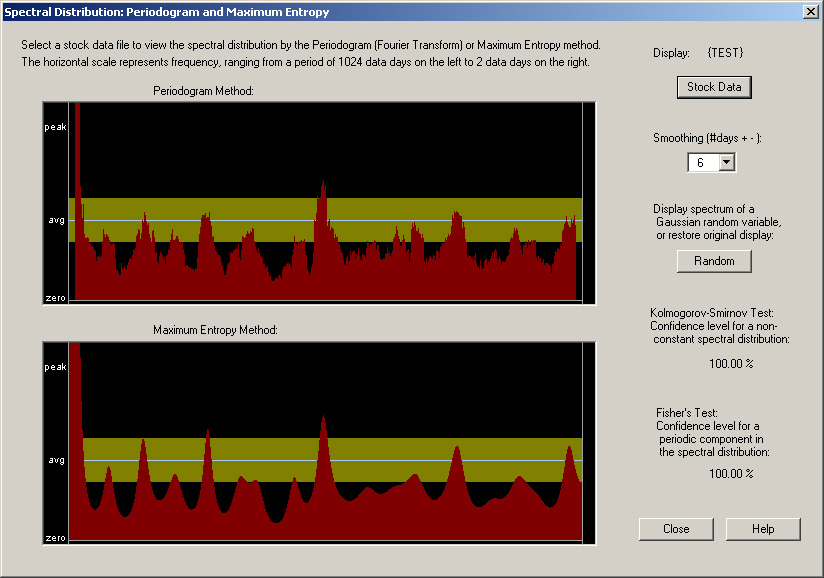
The pure sine wave is the extreme peak at the low-frequency end of the scale, which runs completely off the vertical scale. This kind of single-frequency signal would never occur in real financial data. Also notice that the two statistical tests indicate the presence of a non-random signal and a cyclic signal, with 100% confidence.
References
Peter J. Brockwell & Richard A. Davis, Time Series: Theory and Methods, 2nd ed., Springer-Verlag, New York (1991)
William H. Press, Saul A. Teukolsky, William T. Vetterling, & Brian P. Flannery (NR),
Numerical Recipes in C, The Art of Scientific Computing, 2nd ed., Cambridge University Press, Cambridge, UK (1992)
return to Demonstrations page